Guangwen Ding | Xiangyun Sun | Lihua Xu*
© 2021 IIETA. This article is published by IIETA and is licensed under the CC BY 4.0 license (http://creativecommons.org/licenses/by/4.0/).
OPEN ACCESS
The failure rate of distribution system at all levels can be reduced effectively by exploring the change law of temperature rise of electrical control switch cabinet (ECSC), and optimizing the design concept of the cooling system. These efforts can significantly promote the coordinated development of grids at all levels. However, the existing studies rarely discuss the temperature rise law under external factors or non-rated conditions. The factors affecting temperature rise have not been fully considered, not to mention the correlations between these factors. Likewise, few scholars have tried to optimize the design of the cooling system. Therefore, this paper carries out a heat flow field analysis on the cooling system of ECSC. Firstly, the design idea of ECSC cooling system was explained, and the design steps of ECSC cooling were presented. Secondly, a mathematical model was established for the motion of ECSC thermal fluid, based on the laws of conservation of mass, momentum, and energy. Thirdly, a turbulence model and a porous media model were constructed for ECSC heat flow field analysis, after fully considering multiple factors: the compressibility of the fluid, the construction of a special yet feasible problem, the precision requirement, the computing capacity, and the time limit. Finally, the uniformity of the flow field was measured by parameters like mean speed, coefficient of speed fluctuation, and cloud map of speed, the results of ECSC heat flow field analysis were obtained, and useful suggestions were provided for structural optimization.
heat flow field analysis, electrical control switch cabinet (ECSC), cooling system
Following the requirements on electrical wiring, electrical control switch cabinet (ECSC) is a closed or semi-closed metal cabinet containing switching equipment, measuring instruments, and auxiliary equipment, to protect the safety people and surrounding equipment [1-7]. Step-up and step-down distribution systems are an important link of high-voltage supply side and low-voltage user side. ECSC, with core functions like power distribution, control, and transmission protection, is essential to distribution systems at all levels [8-15]. 40% of distribution system accidents are related to the temperature rise of the switch cabinet. If the equipment operates at a high temperature for a long time, the operation of the distribution system will no longer be stable, and overheating may lead to serious combustion accidents [16-22]. The failure rate of distribution system at all levels can be reduced effectively by exploring the change law of temperature rise of ECSC, and optimizing the design concept of the cooling system. These efforts can significantly promote the coordinated development of grids at all levels.
The cooling of the carrier circuit is the key to ECSC design. Zhang et al. [23] introduced the thermal conduction differential equation, Navier-Stokes equations, and radiation heat transfer equation to build a multi-physical field coupling mathematical model of the switch cabinet cooling problem, mathematically modeled the three-dimensional (3D) temperature field and flow field of KYN28A-12 switch cabinet, and conducted calculation by finite-volume method. In industrial applications without cooling devices, thermal conditions in the switch cabinet are also affected by natural convection and radiation heat transfer. Frank et al. [24] enhanced the opensource library Open FOAM to simulate the temperature field of air in the cabinet, adopted Menter's Shear Stress Transport (SST) model to depict the natural convective heat exchange of turbulence, utilized surface-to-surface model to illustrate radiation heat transfer, computed view factors with Monte-Carlo algorithm, and tested Rayleigh–Bénard convection in a cavity. Finally, the numerical results of different flow models were compared with the measured data in the literature, and the correlations between the two sets of data were evaluated. According to the infrared radiation theory, Yan et al. [25] established thermal radiation models of the inner surface of the outer casing induced by the overheating of a single or multiple failed elements in the control cabinet, respectively, obtained the distribution of the total heat flow in the casing, built a three-dimensional (3D) heat transfer model of the heating casing, and determined the overheating temperature and position of failed parts in the cabinet. Drawing on the idea of SAND (Simultaneous Analysis and Design), Zhang et al. [26] converted the analysis of ECSC system into an optimization problem, introduced the Krig model as an alternative model of the output variables of each subsystem, initialized the Kirg model based on sparse sample points. The established model can greatly reduce the number of subsystem simulations needed for system analysis. Their method was proved valid against a typical thermoelectric coupling problem. Based on the existing data of fire tests, Macheret and Amico [27] modeled the peak heat release rate (HRR) of vertical cabinet fire, determined the proportionality of peak HRR and combustion energy release under unlimited oxygen supply, and further correlated the energy with the initial fuel load of the cabinet.
To sum up, some scholars have studied and expounded the heat dissipation performance of ECSC, laying a solid basis for our research. The existing studies have solved ECSC temperature distribution accurately. However, rarely has any researcher discussed the temperature rise law under external factors, or non-rated working conditions. The factors affecting temperature rise have not been fully considered, not to mention the correlations between these factors. Likewise, few scholars have tried to optimize the design of the cooling system. Therefore, this paper carries out a heat flow field analysis on ECSC cooling system. Section 2 explains the design idea of ECSC cooling system, and gives the design steps of ECSC cooling. Section 3 establishes a mathematical model for the motion of ECSC thermal fluid, based on the laws of conservation of mass, momentum, and energy, and constructs a turbulence model and a porous media model for ECSC heat flow field analysis, after fully considering the following factors: the compressibility of the fluid, the construction of a special yet feasible problem, the precision requirement, the computing capacity, and the time limit. Section 4 measures the uniformity of the flow field by parameters like mean speed, coefficient of speed fluctuation, and cloud map of speed. Through experiments, the results of ECSC heat flow field analysis were obtained, and useful suggestions were provided for structural optimization.
Figure 1. Surface heating power coefficients
Figure 1 shows the surface heating power coefficient of each cooling mode. ECSC cooling mode is selected preliminarily based on the coefficient value. When the mean cooling density falls in [0.08, 0.31], forced air cooling should be adopted to meet the requirements of cooling design. Figure 2 gives the general steps of ECSC cooling design.
Traditionally, heat flow and heat transfer problems are solved experimentally and theoretically. But the traditional solutions only apply to some simple working conditions, due to their limited applicable scope or the constraints of test methods/conditions. To predict the heat flow field of ECSC cooling quickly and accurately, this paper numerically simulates the heat flow field of ECSC with wind cooling devices, using the computational fluid dynamics (CFD) software.
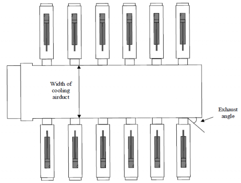
Figure 3 shows the internal cooling structure of ECSC. The inlets of the ventilation system are installed on the front and rear sides of ECSC. An axial flow fan is mounted on the top. There are shutters on the cabinet door. The heat released by the internal components of ECSC is discharged outward from the exhaust of the cooling airduct.
Figure 2. Steps of ECSC cooling design
Figure 3. Internal cooling structure of ECSC
The computational domain of the thermal fluid in ECSC was meshed by Ansys ICEM CFD. The switch cabinet was divided into regular hexahedrons, while the inlets and outlet were modeled by unstructured tetrahedrons. The interface between the two kinds of grids was set to the interior interface, such that the data can be transmitted effectively across computational domains. Then, a mathematical model for the motion of ECSC thermal fluid was established, based on the laws of conservation of mass, momentum, and energy.
Based on the law of conservation of mass, it is possible to construct the mass conservation equation of ECSC, which can characterize the net mass of the microbody flowing into ECSC in the same time interval. The mass equals the mass increment of the fluid microbody in ECSC per unit time. Let σ be fluid density; τ be time; o be the fluid speed vector; o, p and q be the component of the fluid speed vector in directions a, b, and c, respectively. Then, we have:
$\frac{\partial \sigma }{\partial \tau }+\frac{\partial \left( \sigma o \right)}{\partial a}+\frac{\partial \left( \sigma p \right)}{\partial b}+\frac{\partial \left( \sigma q \right)}{\partial c}=0$ (1)
If ECSC thermal fluid is incompressible, its density σ can be regraded as a constant. Then, the above mass conservation equation can be simplified as:
$\frac{\partial o}{\partial a}+\frac{\partial p}{\partial b}+\frac{\partial q}{\partial c}=0$ (2)
The momentum conservation equation measures the time change rate of the thermal fluid momentum in ECSC microbody by the sum of all external forces acting on the microbody. Here, ECSC thermal fluid is viewed as an incompressible fluid with a constant viscosity. Let V be the pressure on the microbody of ECSC thermal fluid; σ be fluid density; λ be kinetic viscosity. Then, the momentum conservation equation can be simplified as:
$\sigma \left( \frac{\partial o}{\partial \tau }+o\frac{\partial o}{\partial a}+p\frac{\partial o}{\partial b}+q\frac{\partial o}{\partial c} \right)=\sigma {{G}_{a}}-\frac{\partial V}{\partial a}+\lambda \left( \frac{{{\partial }^{2}}o}{\partial {{a}^{2}}}+\frac{{{\partial }^{2}}o}{\partial {{b}^{2}}}+\frac{{{\partial }^{2}}o}{\partial {{c}^{2}}} \right)$ (3)
$\sigma \left( \frac{\partial p}{\partial \tau }+o\frac{\partial p}{\partial a}+p\frac{\partial p}{\partial b}+q\frac{\partial p}{\partial c} \right)=\sigma {{G}_{b}}-\frac{\partial V}{\partial b}+\lambda \left( \frac{{{\partial }^{2}}p}{\partial {{a}^{2}}}+\frac{{{\partial }^{2}}p}{\partial {{b}^{2}}}+\frac{{{\partial }^{2}}v}{\partial {{c}^{2}}} \right)$ (4)
$\sigma \left( \frac{\partial q}{\partial \tau }+o\frac{\partial q}{\partial a}+p\frac{\partial q}{\partial b}+q\frac{\partial q}{\partial c} \right)=\sigma {{G}_{c}}-\frac{\partial V}{\partial c}+\lambda \left( \frac{{{\partial }^{2}}q}{\partial {{a}^{2}}}+\frac{{{\partial }^{2}}q}{\partial {{b}^{2}}}+\frac{{{\partial }^{2}}q}{\partial {{c}^{2}}} \right)$ (5)
The energy conservation equation measures the increasing rate of the energy for the microbody entering ECSC by the work of body force and surface force on the microbody plus the net heat flow. Let χ be the specific heat capacity; φ be temperature; Ψ be the heat transfer coefficient of the fluid; Rφ be the viscous dissipation term. Then, we have:
$\begin{align} & \frac{\partial \left( \sigma \phi \right)}{\partial \tau }+\frac{\partial \left( \sigma o\phi \right)}{\partial a}+\frac{\partial \left( \sigma p\phi \right)}{\partial b}+\frac{\partial \left( \sigma q\phi \right)}{\partial c}= \\ & \frac{\partial }{\partial a}\left( \frac{\Psi }{{{\chi }_{v}}}\frac{\partial \phi }{\partial a} \right)+\frac{\partial }{\partial b}\left( \frac{\Psi }{{{\chi }_{v}}}\frac{\partial \phi }{\partial b} \right)+\frac{\partial }{\partial c}\left( \frac{\Psi }{{{\chi }_{v}}}\frac{\partial \phi }{\partial c} \right)+{{R}_{\phi }} \\\end{align}$ (6)
Under different initial conditions and boundary conditions, the viscous fluid could belong to two different flow states: the laminar state, and the turbulent state. In ECSC with air cooling devices, when the wind speed provided by the devices is relatively slow, the internal thermal fluid flows in different layers, forming a laminar flow. As the wind speed increases, the streamline of the internal thermal fluid swings like a wave, with a growth of swinging frequency and amplitude, forming a transitional flow. When the wind speed is relatively fast, the laminar flow of the internal thermal fluid is damaged, the streamline becomes illegible. In this case, adjacent layers slide against and mix with each other, and the thermal fluid moves irregularly, forming a turbulent flow. This paper relies on the critical Reynolds number RE to differentiate between laminate flow and turbulent flow in ECSC. Let σ be the density of the internal thermal fluid; υ be fluid speed; e be feature length; λ be kinetic viscosity. Then, we have:
$RE=\frac{\sigma \upsilon e}{\lambda }$ (7)
For ECSC with air cooling devices, if RE≥2300, the internal thermal fluid forms a turbulent flow; if RE≤2300, the fluid forms a laminar flow. In this paper, the hot gas flow inside ECSC is very complex, but mostly belongs to the turbulent state. Let OV be the orifice area; WC be the wetted perimeter. Since the outlet of ECSC is rectangular, the feature length d equals EF:
${{E}_{F}}=4\frac{OV}{WC}$ (8)
The turbulence model for ECSC heat flow field analysis should be selected in the light of various factors: the compressibility of the fluid, the construction of a special yet feasible problem, the precision requirement, the computing capacity, and the time limit. Considering the applicable scopes and advantages of multiple turbulence models, this paper chooses the renormalization group theory k-epsilon (RNG k-ε) model to simulate the flow problem of ECSC heat flow field. Extended from the standard k-ε model, the RNG k-ε turbulence model thoroughly considers turbulent vortexes, improves the simulation precision facing these vortexes, and provides an analytical formula containing low RE flow viscosity. As a result, the model is highly credible and precise in depicting a wide range of flows. In the RNG k-ε turbulence model, k refers to the kinetic energy of turbulent pulsation, and ε is the diffusion rate of turbulent pulsation. The two parameters are adopted by the model to close the control equations. Let σ be fluid density; oi and oj(i,j=1,2,3) be the time-mean speed components; ai and aj be the components on each axis; xk and xε be the Prandtl number of k and ε, respectively (k=ε=1.4); D1ε and D2ε be the turbulence model coefficients (D1ε=1.4; D2ε=1.7); δ is the dimensionless parameter; Φij be the time-mean strain rate; Hk be the term produced by the turbulent energy k induced by the mean speed gradient; λi be the turbulent viscosity. Then, we have:
$\frac{\partial k}{\partial \tau }+{{o}_{i}}\frac{\partial k}{\partial {{a}_{i}}}=\frac{\partial }{\partial {{a}_{j}}}\left[ {{\beta }_{l}}\frac{{{\lambda }_{EQ}}}{\sigma }\frac{\partial k}{\partial {{a}_{j}}} \right]+\frac{{{H}_{l}}}{\sigma }-\varepsilon $ (9)
$\begin{align}& \frac{\partial \varepsilon }{\partial \tau }+{{o}_{i}}\frac{\partial \varepsilon }{\partial {{a}_{i}}}=\frac{\partial }{\partial {{a}_{j}}}\left[ \left( {{\beta }_{\varepsilon }}\frac{{{\lambda }_{EQ}}}{\sigma } \right)\frac{\partial \varepsilon }{\partial {{a}_{j}}} \right]+ \\ & D_{1\varepsilon }^{*}\frac{\varepsilon }{k\sigma }{{H}_{l}}-{{D}_{2\varepsilon }}\sigma \frac{{{\varepsilon }^{2}}}{l} \\\end{align}$ (10)
where,
$D_{1\varepsilon }^{*}={{D}_{1\varepsilon }}-\frac{\delta \left( 1-\delta /{{\delta }_{0}} \right)}{1+\alpha {{\delta }^{3}}}$ (11)
δ can be calculated by:
$\delta =\sqrt{2{{\Phi }_{ij}}\cdot {{\Phi }_{ij}}}\frac{k}{\varepsilon }$ (12)
Φij can be calculated by:
${{\Phi }_{ij}}=\frac{1}{2}\left( \frac{\partial {{o}_{i}}}{\partial {{a}_{j}}}+\frac{\partial {{o}_{j}}}{\partial {{a}_{i}}} \right)$ (13)
Hk can be calculated by:
${{H}_{k}}={{\lambda }_{\tau }}\left( \frac{\partial {{o}_{i}}}{\partial {{a}_{j}}}+\frac{\partial {{o}_{j}}}{\partial {{a}_{i}}} \right)\frac{\partial {{o}_{i}}}{\partial {{a}_{j}}}$ (14)
λτ can be calculated by:
${{\lambda }_{\tau }}=\sigma {{D}_{\lambda }}\frac{{{k}^{2}}}{\varepsilon }$ (15)
The equivalent viscosity coefficient is represented by λEQ==λ+λτ; constants Dλ, δ0 and α are empirically set to 0.086, 4.7, and 0.015, respectively.
In ECSC, the maximum boundary dimensions are adopted for the cabinet, elements, wiring ducts, and other accessories. Generally, the ventilation scheme consists of inlets below the front door, and an outlet above the front door, with no inlet or outlet at the rear door. ECSC thermal fluid can pass through the elements and cables in any direction. Hence, the wiring ducts and elements can be simplified as a whole into a porous medium. The porous medium model can be viewed as the momentum equation, plus two source terms, namely, viscous loss and inertial loss. Let |υ| be the hot wind speed of ECSC; QE and QF be the specified coefficient matrices. Then, the (a,b,c) momentum source term Ri in direction i can be expressed as:
${{R}_{i}}=\sum\limits_{j=1}^{3}{Q{{E}_{ij}}o{{\upsilon }_{j}}}+\sum\limits_{j=1}^{3}{Q{{F}_{ij}}\left| {{\upsilon }_{j}} \right|{{\upsilon }_{j}}}$ (16)
Let β be the penetration rate; D* be the inertial resistance coefficient. If the elements are arranged simply in an isotropic manner. Formula (16) can be simplified as:
${{R}_{i}}=\frac{\lambda }{\beta }{{\upsilon }_{j}}+{{D}^{\text{*}}}\frac{1}{2}\sigma \left| {{\upsilon }_{j}} \right|{{\upsilon }_{j}}$ (17)
Let ZJV and ϕ be the mean width and porosity of elements, respectively. Then, the viscous resistance coefficient 1/β can be calculated by:
$\beta =\frac{ZJ_{V}^{2}}{150}\frac{{{\varphi }^{3}}}{{{\left( 1-\varphi \right)}^{2}}}$ (18)
The inertial resistance coefficient D* can be calculated by:
${{D}_{2}}=\frac{3.5}{Z{{J}_{V}}}\frac{\left( 1-\varphi \right)}{{{\varphi }^{3}}}$ (19)
The hot wind speed in ECSC is a key constraint of the cooling performance of the switch cabinet. After entering the cabinet, the uneven distribution of the hot wind directly leads to the uniform cooling of elements, and significantly undermines the cooling performance of the cabinet. To better explore the uniformity of ECSC heat flow field, the uniformity of the flow field was measured by parameters like mean speed, coefficient of speed fluctuation, and cloud map of speed. The mean speed refers to the mean gas speed observed at monitoring points. As an indicator of gas flow intensity inside the cabinet, the faster the mean speed, the wider the range of gas flow, and the better the cooling performance.
The coefficient of speed fluctuation SP characterizes the violence of fluid speed change in ECSC heat flow field. When the gas in ECSC heat flow field is distributed very unevenly, the SP value will be relatively large, a sign of the poor cooling performance of the cabinet. The SP value can be calculated by:
$\begin{align}& SP=\frac{{{\chi }_{\upsilon }}}{\upsilon }\times 100{\scriptstyle{}^{0}/{}_{0}} \\ & =\frac{\sqrt{\frac{1}{m-1}\sum\nolimits_{i=1}^{m}{{{\left( {{\upsilon }_{i}}-{{\upsilon }^{*}} \right)}^{2}}}}}{{{\upsilon }^{*}}}\times 100{\scriptstyle{}^{0}/{}_{0}} \\\end{align}$ (20)
where, χυ is the standard deviation of the hot wind speeds observed at all monitoring points on the same plane; υ* be the mean of these speeds; m be the number of monitoring points.
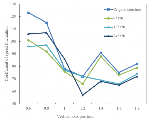
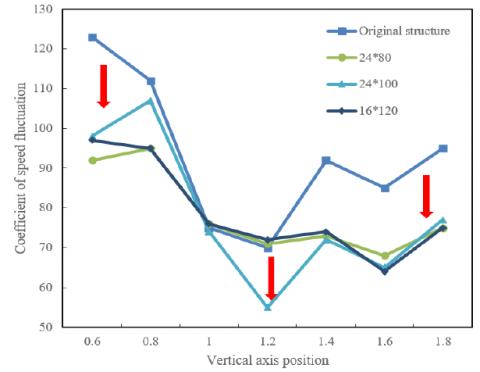
After adding inlet hoods to ECSC, the heat flow field in ECSC at seven different horizontal cross-sections were simulated: 0.6, 0.8, 1, 1.2, 1.4, 1.6, and 1.8m. These horizontal cross-sections reflect the spatial heat flow field situation near the inlets of ECSC. Based on the temperature collected from the monitoring points, the curves of the coefficients of speed fluctuations for thermal fluid on the 7 horizontal cross-sections were plotted and shown in Figure 4. It can be learned that, on the horizontal cross-section of the height 0.8, the coefficients of speed fluctuations for thermal fluid under different hood settings were basically the same with that of the original structure. The coefficients of speed fluctuations in the scheme of 24°/100mm declined the greatest from the levels of the original structure. Hence, this scheme was adopted for the structural optimization of inlet hoods.
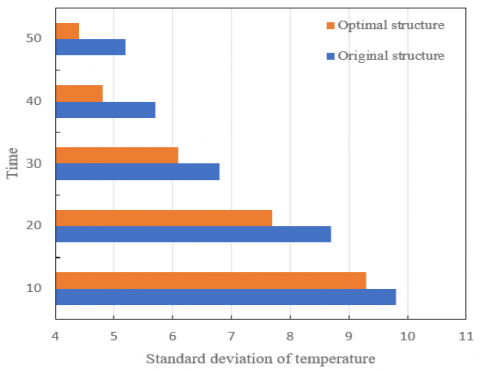
Figure 5 shows the standard deviation of temperature on vertical cross-sections relative to the central axis between the optimal structure and the original structure. The standard deviation of temperature can characterize the uniformity of the temperature field inside ECSC. It can be observed that the standard deviation of temperature between the two structures gradually reduced with the growing operation time of the cabinet. Thus, ECSC temperature tends to be uniform, as the cool wind provided by the cooling system continues to flow around.
This paper tests and controls the temperature at key parts of ECSC. The monitored values are summarized in Tables 1-3.
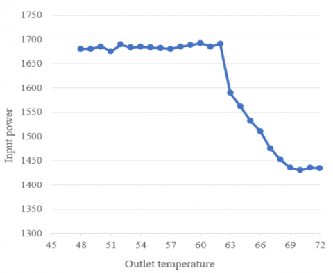
In the sealed environment of ECSC, the temperature constantly rises. Figure 6 shows the variation of input power with outlet temperatures.
Figure 7 compares the mean cooling efficiencies at different working conditions before and after the structural optimization of the cabinet. It can be seen that, when the outlet temperature fell in [40°C, 60°C], the mean cooling efficiency of the cabinet remained stable. When the temperature surpassed 65°C, the mean cooling efficiency of the cabinet started to drop.
(1)
(2)
Figure 4. Coefficients of speed fluctuations for thermal fluid on the horizontal cross-section under different hood settings
Figure 5. Standard deviation of temperature on vertical cross-sections relative to the central axis
Figure 6. Variation of input power with outlet temperatures
Figure 7. Mean cooling efficiencies at different working conditions before and after the structural optimization of the cabinet
Table 1. Cylinder manifold temperatures
|
Bus cylinder manifold Temperature |
Cylinder manifold A |
Cylinder manifold B |
Cylinder manifold C |
|
124.515oC |
115.4127oC |
113.4758oC |
|
|
Cable cylinder manifold Temperature |
Cylinder manifold A |
Cylinder manifold B |
Cylinder manifold C |
|
103.2814oC |
105.4962oC |
101.0825oC |
Table 2. Fixed contact temperatures
|
Bus fixed contact Temperature |
Contact A |
Contact B |
Contact C |
|
116.8512oC |
118.2953oC |
114.1852oC |
|
|
Cable fixed contact Temperature |
Contact A |
Contact B |
Contact C |
|
105.1957oC |
108.3296oC |
105.4953oC |
Table 3. Fixed contact temperature rises
|
|
Time /h |
1 |
2 |
3 |
4 |
5 |
6 |
|
Bus fixed contact Temperature rise |
Phase A |
9.2 |
43.2 |
67.4 |
78.5 |
82.6 |
85.2 |
|
Phase B |
9.8 |
44.8 |
54.6 |
66.8 |
73.8 |
75.8 |
|
|
Phase C |
7.8 |
45.2 |
58.4 |
68.5 |
73.1 |
76.2 |
|
|
Cable fixed contact Temperature rise |
Phase A |
13.8 |
45.2 |
63.8 |
74.7 |
73.6 |
75.9 |
|
Phase B |
14.5 |
42.9 |
53.6 |
64.2 |
66.5 |
68.4 |
|
|
Phase C |
12.8 |
43.8 |
52.1 |
65.9 |
68.3 |
66.2 |
Table 4. Mean cooling efficiencies at different working conditions before and after the structural optimization of the cabinet
|
Wind speed |
3.1 |
3.4 |
3.2 |
6.3 |
8.1 |
Mean/(%) |
|
|
Simulated heat sources |
815 |
1637 |
2415 |
2435 |
2484 |
||
|
Mean cooling efficiency |
Oil cooling cabinet |
51.29 |
29.16 |
22.51 |
24.85 |
24.75 |
30.25 |
|
Air cooling cabinet |
32.58 |
19.47 |
15.42 |
16.48 |
19.75 |
18.59 |
|
Figure 8. Experimental values vs. theoretical values of the original ECSC under different working conditions
Figure 9. Experimental values vs. theoretical values of the optimal ECSC under different working conditions
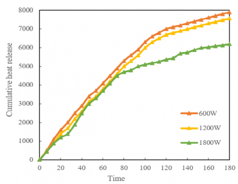
According to the experimental results, the authors computed the mean cooling efficiencies at different working conditions before and after the structural optimization of the cabinet (Table 4). Figures 8 and 9 compare the experimental values with the theoretical values. To further demonstrate the cooling performance of ECSC, the cumulative heat releases of the cabinet before and after optimization measured through experiments were compared with the modeling results.
It can be learned from the figures that, under the same working condition, the optimized ECSC was more efficient in cooling than the original ECSC. Compared with the original ECSC, the optimal ECSC on average increased the cooling efficiency by 16.15%. After optimization, the mean cooling efficiency of ECSC was 28.54%. By contrast, the mean cooling efficiency of air cooling cabinet was 12.39%. Hence, structural optimization improves the cooling performance of the cabinet.
Based on heat flow field analysis, this paper probes deep into ECSC cooling system. The authors detailed the design idea of ECSC cooling system, as well as the design steps of ECSC cooling. Drawing on the laws of conservation of mass, momentum, and energy, a mathematical model was established for the motion of ECSC thermal fluid. On this basis, a turbulence model and a porous media model were constructed for ECSC heat flow field analysis, through full consideration of factors like the compressibility of the fluid, the construction of a special yet feasible problem, the precision requirement, the computing capacity, and the time limit. In addition, the uniformity of the flow field was measured by parameters like mean speed, coefficient of speed fluctuation, and cloud map of speed. The coefficients of speed fluctuations for thermal fluid on the horizontal cross-section were compared under different hood settings. In this way, the optimal inlet hood setting was determined for structural optimization of ECSC. Through experiments, the authors tested and controlled the temperature at key parts of ECSC, plotted the variation of input power with outlet temperatures, and computed the mean cooling efficiencies at different working conditions before and after the structural optimization of the cabinet. The experimental results demonstrate that the structural optimization promotes the cooling efficiency of ECSC. Finally, the experimental values of the optimal ECSC under different working conditions were compared with theoretical values, and suggestions were put forward to improve structural optimization.
[1] Gao, J., Kou, J., Zhao, Y., Luo, J., Xu, A. (2019). Research and development of partial discharge anti disturbance system for switch cabinet. In 2019 Chinese Control and Decision Conference (CCDC), pp. 516-519. https://doi.org/10.1109/CCDC.2019.8832488
[2] Matthies, T. (2019). Modern I/O systems take into account the change in the switch cabinet construction: More space in the switch cabinet. Konstruktion, 2019: 11-12.
[3] Joppen, R., von Enzberg, S., Kühn, A., Dumitrescu, R. (2019). Investment decisions in the context of digitization using switch cabinet construction as an example. ZWF Zeitschrift fuer Wirtschaftlichen Fabrikbetrieb, 114(7-8): 483-487.
[4] Le, J., Zhou, Q., Wang, C., Yang, Z.C., Zhang, H. (2019). Development of an over-temperature supervising system of switch cabinet based on gas sensing technology. International Journal of Emerging Electric Power Systems, 20(2). https://doi.org/10.1515/ijeeps-2018-0068
[5] Huang, X.B., Xue, Z.P., Tian, Y., Jiang, B.T., Chen, L. (2019). Early thermal fault warning strategy of high voltage switch cabinet and its application. Dianli Zidonghua Shebei/Electric Power Automation Equipment, 39(7): 181-187.
[6] Fu, C.Z., Si, W.R., Huang, H., Chen, L., Gao, Q.J., Shi, C. B., Wang, C. (2018). Research on a detection and recognition algorithm for high-voltage switch cabinet based on deep learning with an improved YOLOv2 Network. In 2018 11th International Conference on Intelligent Computation Technology and Automation (ICICTA), pp. 346-350. https://doi.org/10.1109/ICICTA.2018.00085
[7] Sun, Y., Song, J., Guo, H., Li, S., Li, J., Wang, Z. (2021). The state evaluation method of distribution switch cabinet based on improved matter-element extension. In E3S Web of Conferences, 236. https://doi.org/10.1051/e3sconf/202123601011
[8] Frische-Meier, J. (2020). Support in switch cabinet construction with software-assisted tool: Assistance systems for machine operators increase efficiency. Konstruktion, 2020(4): 24-27.
[9] Teng, G., Wang, Y., Peng, J., Qi, D. (2020). Detection-free framework for cabinet switch state recognition. In 2020 International Conference on Image, Video Processing and Artificial Intelligence, 11584, pp. 1158409. https://doi.org/10.1117/12.2579437
[10] Großmann, C., Kuhlenkötter, B., Kutschinski, J., Linsinger, M. (2018). Assembly in switch cabinet construction: Research cooperation shows how it is done in a cheaper and faster manner. Konstruktion, 2018(11-12): 18-20.
[11] Wang, F., Han, S., Cao, B. (2018). A hierarchical fuzzy comprehensive evaluation algorithm for running state of a 6 kV (10 kV) power switch cabinet. Mathematical Problems in Engineering, 2018. https://doi.org/10.1155/2018/4517279
[12] Jiang, Y., Huang, Y., Liao, Y. (2016). A partial discharge monitoring system for high voltage switch cabinet using UV sensors. International Journal of Simulation--Systems, Science & Technology, 17(14): 14.1-14.4. https://doi.org/10.5013/IJSSST.a.17.14.14
[13] Li, P., Huang, D.C., Ruan, J.J., Niu, X., Zhu, C. (2015). Electromagnetic interference on secondary smart devices caused by breaking 10 k V switch cabinet. Power System Technology, 39(1): 110-117.
[14] Schreiber, A. (2020). How one makes the "process chain of switch cabinet construction" more efficient: Designing switch cabinet construction together. Konstruktion, 2020(9): 54-56.
[15] Yin, K., Huang, X., Zhong, T., Chen, Q., Tong, X. (2021). Modular substation intelligent control cabinet temperature control system. In Journal of Physics: Conference Series, 2005(1): 012092.
[16] Lu, L., Wang, W., Li, G., Mitrouchev, P. (2019). Study on the detection system for electric control cabinet. In International Workshop of Advanced Manufacturing and Automation, 29-36. https://doi.org/10.1007/978-981-15-2341-0_4
[17] Taur, A., Badave, S.M., Padmanaban, S., Bhaskar, M.S., Ramachandaramurthy, V.K., Holm-Nielsen, J.B. (2019). Testing of local control cabinet in gas insulated switchgear using design of simulation kit-Revista. In 2019 IEEE 13th International Conference on Compatibility, Power Electronics and Power Engineering (CPE-POWERENG), pp. 1-5. https://doi.org/10.1109/CPE.2019.8862400
[18] Mou, X., Leng, C., Zhou, X., Cai, Y. (2018). State recognition of electric control cabinet switches based on cnns. In 2018 IEEE 3rd International Conference on Image, Vision and Computing (ICIVC), pp. 183-187. https://doi.org/10.1109/ICIVC.2018.8492853
[19] Yang, L., Wang, Y., Liu, H., Yan, G., Kou, W. (2014). Infrared identification of internal overheating components inside an electric control cabinet by inverse heat transfer problem. In International Symposium on Optoelectronic Technology and Application 2014: Infrared Technology and Applications, 9300: 930002. https://doi.org/10.1117/12.2072030
[20] Duan, J.D., Ye, B., Zhang, Q.S., Fan, H. (2014). Online contact temperature monitoring and control system based on finned radiator and ZigBee for switch cabinet. Electric Power Automation Equipment, 34(7): 157-162.
[21] Ordonez, J.C., Vargas, J.V.C., Hovsapian, R. (2008). Modeling and simulation of the thermal and psychrometric transient response of all-electric ships, Internal compartments and cabinets. Simulation, 84(8-9): 427-439. https://doi.org/10.1177/0037549708097421
[22] Rustogi, S., Gupta, A. (2004). Modeling the dynamic behavior of electrical cabinets and control panels: experimental and analytical results. Journal of Structural Engineering, 130(3): 511-519.
[23] Zhang, J.M., Gao, C., Feng, H., Yan, G.C., Zhao, F., Yuan, D.L., Zhao, H.F. (2011). A coupled three-dimensional fluid-thermal fields analysis of KYN28A-12 switch cabinet. In 2011 1st International Conference on Electric Power Equipment-Switching Technology, pp. 466-470. https://doi.org/10.1109/ICEPE-ST.2011.6123032
[24] Frank, A., Heidemann, W., Spindler, K. (2019). Electronic component cooling inside switch cabinets: combined radiation and natural convection heat transfer. Heat and Mass Transfer, 55(3): 699-709.
[25] Yan, G.H., Yang, L., Fan, C.L. (2012). Three-dimensional inverse problem identification of thermal defect temperature and the position of fault components in the electrical control cabinet based on infrared temperature measurement. Infrared and Laser Engineering, 41(11): 2909-2915.
[26] Zhang, Z., Yu, F., Wang, Q.Y., Du, S.P. (2017). Thermal-electric coupling systems analysis of electronic cabinets with consideration of numerical noises. Journal of Vibration and Shock, 36(13): 214-222. https://doi.org/10.13465/j.cnki.jvs.2017.13.034
[27] Macheret, P., Amico, P.J. (2011). Evaluation of heat release rates of vertical electrical cabinet fires. International Topical Meeting on Probabilistic Safety Assessment and Analysis 2011, 2: 983-997.