Haining Gao* | Hongdan Shen | Lei Yu | Yinling Wang | Yong Yang | Shouchen Yan | Yingjie Hu
© 2021 IIETA. This article is published by IIETA and is licensed under the CC BY 4.0 license (http://creativecommons.org/licenses/by/4.0/).
OPEN ACCESS
During high-speed cutting, the tool quality is threatened by a high cutting temperature, and severe wear. Traditionally, these threats are handled by tool replacement, which pushes up the economic cost of production and manufacturing. This paper explores the frictional wear detection of hard alloy tool material during high-speed cutting. Based on the theory of wave motion, the wear process of hard alloy tool material during high-speed cutting was modelled mathematically, and the wear mechanism was analyzed. To reduce the interference of weakly important features, the authors presented a method to analyze the feature importance and an approach to identify the frictional wear of tools, under the high-dimensional small dataset about the monitoring signals of tool material wear. Through experiments, the proposed algorithm was proved feasible in identifying the wear of hard alloy tool material during high-speed cutting. The research provides a theoretical guide for improving the production techniques for cutting of hard alloy material.
high-speed cutting, hard alloy tool, frictional wear of tool material
In the age of Industry 4.0, the digital transformation of manufacturing is featured by the automation, intelligence, high precision, and integration of traditional manufacturing industry. The industrial products need to meet an increasingly high demand of performance and quality [1-5]. During high-speed cutting, the tool quality is often threatened by a high cutting temperature, and severe wear. These threats severely restrain the improvement of production efficiency, processing precision, and surface quality of products [6-10]. To guarantee processing quality, the traditional solution is rather conservative: tool replacement. But this approach pushes up the economic cost of production and manufacturing [11-17]. For more efficient production and cost-effective processing, it is necessary to theoretically model the frictional wear of tools, carry out microscopic detection, and implement simulation analysis [18-21], aiming to provide a theoretical guide for improving the production techniques for cutting of hard alloy material.
Industrial applications should consider the applicability, ease of implementation, and cost effectiveness of process optimization. Zhang and Xu [22] developed a Gaussian process regression (GPR) model to predict three cutting parameters, namely, cutting force, surface roughness, and tool life, during high-speed turning, based on cutting speed, feed rate, and cutting depth. Tool wear is the main reason for the failure of tool acceleration during the milling of aluminum alloys. The milling process is intermittent. The periodic cutting force directly affects cutting heat and tool wear. Focusing on the impact of cutting force on tool wear, Meng et al. [23] analyzed the change law of cutting force with cutting parameters, examined the influence of milling length over the width of the flank surface wear zone, and explored the tool wear mechanism during high-speed milling of aluminum alloy pressure castings, in the light of the effect of the cutting force. Chaus et al. [24] studied the wear resistance and cutting performance of non-coated and coated high-speed steel ball head millers, and observed some surface defects in the exposed carbides in steel substrate and uncoated tool. Javidikia et al. [25] discussed the impact of cutting environment and conditions on the tool wear and residual stress caused by AA6061-T6 orthogonal cutting, developed a two-dimensional (2D) finite element model (FEM) to predict tool wear and residual stress, and verified the 2D FEM with the experimentally measured data on processing force, tool wear, and residual stress. Laser-assisted high-speed milling is a subtractive technique, which thermally softens the material surface to improve the workability of the material under a high removal rate, improve surface finish, and extend tool life. Yasmin et al. [26] adopted the response surface method to investigate how ultrasonic induced droplet cutting fluid affects the surface roughness and side wear of 6082 aluminum alloy, and compared it with traditional droplet cutting fluids. The comparison confirms that the laser-assisted high-speed milling using ultrasonic induced droplet cutting fluid applies to high productivity manufacturing, and helps to shorten production time, reduce operating costs, better surface finish, and extend tool life.
The frictional wear detection of hard alloy tool material is a classification task of high-dimensional small samples. Although many researchers have studied different tool states, it remains interesting to discuss the wear mechanism of the tool cutting edge. Further analysis is wanted to recognize tool wear more accurately, using a few monitoring data features of tools under high-speed cutting. Therefore, this paper explores the frictional wear detection of hard alloy tool material during high-speed cutting. Section 2 draws on the theory of wave motion to mathematically model the wear process of hard alloy tool material, and analyze the wear mechanism. Section 3 discusses the feature importance and the frictional wear identification of tools, under the high-dimensional small dataset about the monitoring signals of tool material wear, and manages to eliminate weakly important features. Finally, experiments demonstrate that the proposed algorithm is feasible in identifying the wear of hard alloy tool material during high-speed cutting.
In theory, the life of a cutting tool can be divided into three stages: initial wear I, stable wear II, and severe wear III (Figure 1). During initial wear, new tool wears faster because the cutting edge is not smooth. During stable wear, the tool wears stably and slowly, and the wear amount is approximately linear with time. During severe wear, the tool wear picks up speed until the tool fails.
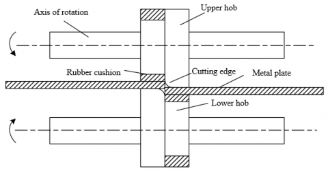
Figure 2 illustrates the high-speed cutting of a rolling shear cutter. During high-speed cutting, the frictional wear of hard alloy tool material largely depends on the target metal plate section. From a microscopic perspective, the action of the tiny particle of the metal plate section on tool material can be viewed as an impact extrusion, followed by relative scraping. From the angle of the forces on tool material, the action process can be simplified as a monistic impact process, with the tiny particle as a mass point and the tool as the receptor. There is a resistance during the interaction between the tiny particles and the tool, for the two parties are not completely detached.
Figure 1. Tool wear curve during the cutting process
Figure 2. High-speed cutting of a rolling shear cutter
The tiny particle of the metal plate section in contact with the tool can be regarded as a rigid body. The mass and position of the particle are denoted by n and t, respectively. Let AC*, AC1 and AC2 be the counter force of the working medium, the force of the metal plate on the rigid body, and the stress wave force, respectively. According to Newton’s laws of motion, the motion equation without considering gravity can be constructed as:
$n \frac{d^{2} t}{d \tau^{2}}=A C_{1}+A C_{2}-A C^{\prime}$ (1)
Since the tool material is a hard alloy, it is possible to build an elastic coefficient model. Let LS be the load stiffness of the tool. Without considering the plastic limit resistance of the tool, the counter force can be calculated by:
$A C^{*}=L S \cdot t$ (2)
At the moment of the high-speed cutting of the metal plate, the sheet section will cause the tool side surface to generate a pressure wave ε0(τ) that is gradually transmitted to the cutter end. After a period of ER/μ, the wave passed to the end will rebound and return to the initial position on the tool side surface. Therefore, within the period of [0, 2ER/μ], there is only one stress wave on the interface between the rigid body and tool material. Let ER be the length of the metal plate; μ be the speed of longitudinal wave; IS be the pressure surface area. Then, the stress wave can be represented by:
$A C_{2}=I S \varepsilon_{0}(\tau)$ (3)
Solving the above stress wave equation, it is possible to obtain the relative speed of the interface between the plate and tool material, i.e., the hourly speed of tool action on the metal plate. Let KN0 be the particle speed of the metal plate; μ be the wave speed; φ be the material density. Then, the speed of relative motion can be calculated by:
$\frac{d t}{d \tau}=K N_{0} \cdot \frac{\varepsilon_{0}(\tau)}{\mu \phi}$ (4)
Before being detached from the target metal plate, the small particle on the metal plate section faces the pressure β1 of the tool material and the viscous resistance of the surrounding materials. Let λ be the coefficient of the viscous resistance of the surrounding materials. Then, we have:
$A C_{1}=\beta_{1}+\beta_{2}$ (5)
$\beta_{2}=\lambda \frac{d^{2} t}{d \tau^{2}}$ (6)
Combining formulas (1)-(5), the following kinetic equation can be obtained:
$(n-\lambda) \frac{d^{2} t}{d \tau^{2}}+I S \phi \mu \frac{d t}{d \tau}+L S \cdot t=I S \phi \mu K N_{0}+\beta_{1}$ (7)
To quantify the tool wear, the wear efficiency, which characterizes the instantaneous energy conversion efficiency, is denoted as ϕ, based on the proposed analysis model. Referring to the scraping depth of the small particle on the metal plate surface into the side of the tool material, the maximum force of the particle on tool material can be calculated by:
$\varepsilon_{\max }=\frac{L S t_{\max }}{I S}$ (8)
Let εmax be the maximum stress of the tool; τ0 be the initial cut amount under cutting pressure; tmax be the maximum insert depth of the small particle; ϕ be the impact efficiency; nf be the mass of a single small particle. Then, the scraping depth of the small particle into the tool material can be calculated by:
$\varphi=\frac{\frac{1}{2} L S \tau_{\text {max }}^{2}}{\frac{1}{2} n_{f} K N_{0}^{2}+\beta_{1} \tau_{0}}$ (9)
Owing to the working features of the high-speed cutting tool, the small particle on the metal plate section directly acts on the tool, and the mass of the rigid particle is so small as to be negligible. Thus, the kinetic Eq. (7) can be rewritten as:
$-\lambda \frac{d^{2} t}{d \tau^{2}}+I S \phi \mu \frac{d t}{d \tau}+L S t=I S \phi \mu K N_{0}+\beta_{1}$ (10)
Let C=ISφμ be the wave drag of the metal plate. Within the period of [0, 2ER/μ], formula (10) can be solved as:
$t(\tau)=\frac{K N_{0}}{S_{1}-S_{2}}\left(r^{s_{1} \tau}-r^{s_{2} \tau}\right)+\frac{C \cdot K N_{0}+\beta_{1}}{L S}$ (11)
where, s1 and s2 can be expressed as:
$s_{1}=\frac{c-\sqrt{C^{2}+4 \lambda L S}}{2 \lambda}, s_{2}=\frac{c+\sqrt{C^{2}+4 \lambda L S}}{2 \lambda}$ (12)
Within the period of [0, 2ER/μ], dt(τ)/dτ>0, i.e., t(τ) monotonically increases. Substituting the time τ=τf=2ER/μ it takes to reach the maximum displacement into formula (12), the maximum action depth tmax of the small particle can be calculated by:
$t_{\max }=\left(\frac{r^{2 Q U s_{1} / \mu}-r^{2 Q U_{2} / \mu}}{s_{1}-s_{2}}+\frac{C}{L S}\right) K N_{0}+\frac{\beta_{1}}{L S}$ (13)
On this basis, the maximum stress of the tool can be calculated by:
$\varepsilon_{\text {max }}=\frac{L S \cdot t_{0}}{I S}=\left[\frac{L S\left(e^{2 Ir_{1} / k}-e^{2 I r_{2} / k}\right)}{I S\left(s_{1}-s_{2}\right)}+\phi \mu\right] K N_{0}+\frac{\beta_{1}}{I S}$ (14)
The high-speed cutting efficiency of the tool can be calculated by:
$\varphi=\frac{\frac{1}{2} L S t_{\max }^{2}}{\frac{1}{2} n_{f} K N_{0}^{2}+\beta_{1} t_{0}}$ (15)
Substituting tmax into formula (15):
$\varphi=\frac{\frac{1}{2} L S\left(\frac{r^{2 Q Us_{1} / d}-r^{2 Q U s_{2} / d}}{s_{1}-s_{2}}+\frac{C}{L S}\right)^{2} K N_{0}^{2}+\frac{\beta_{0}^{2}}{2 L S}+\beta_{1}\left(\frac{r^{2 Q U s_{1} / d}-r^{2 Q Us_{2} / d}}{s_{1}-s_{2}}+\frac{C}{L S}\right)}{\frac{1}{2} n_{f} K N_{0}^{2}+\beta_{1}\left(\frac{r^{2 Q Us_{1} / d}-r^{2 Q Us_{2} / d}}{s_{1}-s_{2}}+\frac{C}{L S}\right) K N_{0}+\frac{\beta_{1}^{2}}{L S}}$ (16)
According to the calculation process of tmax, εmax, and ϕ, the scraping depth of the small particle into cutter material, and the maximum depth of the tool must be minimized, in order to reduce the impact extrusion of the non-smooth small particle on the metal plate section on the tool material.
After examining the state and manifestation of tool material wear during high-speed cutting, this paper further classifies the hard alloy tool wear under high-speed cutting. From the angle of feature importance, Gini importance and Lasso feature importance were evaluated, and the extreme learning machine (ELM) algorithm was adopted to identify the frictional wear of tool material.
This paper extracts the features of each monitoring signal of tool material wear. Since the monitoring signals are rich in features, the frictional wear detection method for tool material is prone to over-fitting, or the identification algorithm faces a high load. Thus, it is necessary to reduce the dimensionality of the high-dimensional monitoring signals. In real applications, the monitoring signals of tool material wear do not obey Gaussian distribution. This limits the performance of common dimensionality reduction approaches like principal component analysis (PCA) and linear discrimination. To eliminate weakly important features, this paper adopts two analysis tools, namely, Gini importance and Lasso feature importance.
The Gini index objectively and intuitively reflects the gap between monitoring signals, and predict, prewarn, and prevent the polarization of attributes between signal samples. Let |K| be the total number of classes; ol(l=1, 2, …|K|) be the proportion of class l samples. The Gini index of the sample set P of the monitoring signals of tool material can be calculated by:
$G N(P)=1-\sum_{l=1}^{|K|} o_{l}^{2}$ (17)
Let x be an attribute of set P; U be the number of classes of set P divided by attribute x. Then, the Gini index of x can be calculated by:
$G N(P, x)=\sum_{u=1}^{U} \frac{\left|P^{u}\right|}{|P|} G N\left(P^{u}\right)$ (18)
Lasso is a compression estimation approach that compresses variable coefficients. By this approach, the variables can be selected, while realizing subset contraction. For sample set P={ai,bi}, i=1,2,3,...,m, the following linear regression model can be established:
$b_{i}=\sum_{j=1}^{o} \zeta_{j} a_{i j}+\sigma_{i}$ (19)
Let τ be the adjustment coefficient; ζ=(ζ1,ζ2,...ζo)T be the least squares method. Then, the Lasso estimation can be defined as:
$\zeta^{\prime}=\operatorname{argmin}\left\{\sum_{i=1}^{m}\left(b_{i}-\sum_{j=1}^{o} \zeta_{j} a_{i j}\right)^{2}\right\}$, s.t. $\sum_{j=1}^{o}\left|\zeta_{j}\right| \leq \tau$ (20)
Let Ωm be the regularization coefficient. Adding the penalty function s.t. Σoj=1|ζj|≤τ as the regularization term into the objective function, we have:
$\zeta_{M}^{\prime}\left(\Omega_{m}\right)=\operatorname{argmin}\left\{\sum_{i=1}^{m}\left(b_{i}-\sum_{j=1}^{o} \zeta_{j} a_{i j}\right)^{2}+\Omega m \sum_{j=1}^{o} \zeta_{j}\right\}$ (21)
For the monitoring signals of tool material wear, the feature importance can be characterized by a weight ζj satisfying the objective function:
$\operatorname{LFI}(i)=\zeta_{j}, j=1,2,3, \ldots ., o$ (22)
After completing the analysis of feature importance, the ELM algorithm was adopted to recognize the frictional wear of tool material. Based on generalized inverse matrix theory, the ELM is a feedforward neural network with a single hidden layer. It is known for strong generalization ability, fast learning speed, and good nonlinear fitting ability.
Suppose there are M nonrepetitive input samples of monitoring signals (ai, τi). Among them, the inputs are denoted as ai=[ai1, ai2, …, aim]T. The corresponding outputs are denoted as τi=[τi1, τi2, …, τim]T. Let xl and yl be the weight and bias of the input layer, respectively; θl be the weight matrix between the l hidden layer nodes and the output nodes; H(xl,yl,ai) be the activation function of the l-th hidden layer node. Then, the ELM model with K hidden layer nodes can output:
$g\left(a_{i}\right)=\sum_{l=1}^{K} \theta_{l} H\left(x_{l}, y_{l}, a_{i}\right)=\tau_{i}, i=1,2, \ldots, M$ (23)
The output can be written as a matrix:
$F \theta=\Pi$ (24)
where,
$F=\left[\begin{array}{ccc}H\left(x_{1}, y_{1}, a_{1}\right) & \cdots & H\left(x_{K}, y_{K}, a_{1}\right) \\ \vdots & \vdots & \vdots \\ H\left(x_{1}, y_{1}, a_{M}\right) & \cdots & H\left(x_{K}, y_{K}, x_{M}\right)\end{array}\right], \theta=\left[\begin{array}{l}\theta_{1}^{T} \\ \vdots \\ \theta_{K}^{T}\end{array}\right], \Pi=\left[\begin{array}{l}\tau_{1}^{T} \\ \vdots \\ \tau_{M}^{T}\end{array}\right]$ (25)
Let a be the regularization parameter. Then, the weight of the ELM output layer can be obtained by the least squares method:
$\zeta=F^{T}\left(\frac{1}{\alpha}+F F^{T}\right)^{-1} \Pi$ (26)
The ELM algorithm was adopted to classify the features of the monitoring signals of tool material wear. The prediction accuracy was calculated. On this basis, the mean prediction accuracy was obtained and outputted, making it possible to recognize the frictional wear of tool material.
The ELM was trained on MATLAB. The training process is illustrated in Figure 3. During the iterative training, the ELM reached the precision requirement in the 9th cycle, when the ELM network error was 0.000392.
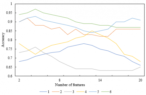
The experimental data come from the processing data produced by numerically controlled machines during high-speed cutting. The experimental dataset contains a total of 312 high-dimensional features. The accuracy of tool wear recognition hinges on the relatively important features. The results of Gini importance analysis are reported in Figure 4. Gini importance analysis eliminates the relatively important features of monitoring signals of tool material wear, retains the highly important features, and thereby reduces the dimensionality of the data on the monitoring signals of tool material wear.
A comparative experiment was designed to verify the effectiveness of our tool wear identification model. The contrastive methods include decision tree (DT), backpropagation (BP) neural network, random forest (RF), support vector machine (SVM), and ELM. Two types of monitoring signals of tool material are covered in the training set: signals of 18 worn tools, and signals of 30 intact tools.
Figure 3. Training process of the proposed classification network
Note: RMSE is short for root mean square error.
Figure 4. Results of Gini importance analysis
Table 1 presents the results of the orthogonal experiments on high-speed cutting in real applications. Based on the results, it is possible to recognize tool wear, and optimize the high-speed cutting parameters.
Table 2 displays the results of tool wear recognition. It can be observed that our model achieved the best recognition accuracy (95.3%); DT (73.22%) and RF (88.83%) performed generally, but did not fail; BP neural network, and SVM failed in tool wear identification.
Among the various features of the dataset, the relatively unimportant data features will undermine the recognition effect of tool wear. Figure 5 gives the results of Lasso feature importance analysis. According to Figures 4 and 5, after the monitoring signals of tool material wear were dimensionally reduced by Gini importance method, all five algorithms performed the best, when the top 7 important features were retained; after the signals were dimensionally reduced by Lasso feature importance method, most methods achieved the best recognition effect, when the top 7 important features were retained, but DT needed to retain the top 10 features, and SVM needed to retain the top 9 features.
Table 1. Results of orthogonal experiments
|
Serial number |
1 |
2 |
3 |
4 |
5 |
|
Cutting speed |
42 |
41 |
43 |
51 |
53 |
|
Feed per tooth |
0.04 |
0.21 |
0.14 |
0.18 |
0.13 |
|
Cutting depth |
0.61 |
1.14 |
1.45 |
1.48 |
0.47 |
|
Cutting width |
5 |
3 |
6 |
5 |
2 |
|
Tool wear amount |
41.295 |
42.195 |
67.495 |
56.289 |
63.185 |
|
Processing time |
1h21m48s |
33m5s |
18m55s |
25m48s |
43m37s |
|
Serial number |
6 |
7 |
8 |
9 |
|
|
Cutting speed |
49 |
58 |
61 |
63 |
|
|
Feed per tooth |
0.13 |
0.07 |
0.11 |
0.16 |
|
|
Cutting depth |
1.15 |
1.13 |
1.49 |
0.47 |
|
|
Cutting width |
4 |
6 |
3 |
5 |
|
|
Tool wear amount |
88.495 |
75.162 |
92.185 |
91.462 |
|
|
Processing time |
25m35s |
33m58s |
24m42s |
39m57s |
|
Table 2. Results of tool wear recognition
|
Algorithm |
DT |
BP neural network |
RF |
SVM |
Our model |
|
Recognition accuracy on worn tools |
72.59% |
1.2% |
85.29% |
1.4% |
91.41% |
|
Recognition accuracy on intact tools |
73.85% |
92.28% |
92.37% |
98.48% |
99.19% |
|
Total accuracy |
73.22% |
46.74% |
88.83% |
49.94% |
95.3% |
Figure 5. Results of Lasso feature importance analysis
Residual analysis was carried out on tool wear recognition based on MATLAB. Table 3 lists the ELM’s residuals and confidence intervals. Figure 6 illustrates the residual distribution.
In Figure 6, the light blue circles are residuals, and the dark blue vertical lines are confidence intervals of residuals. It can be seen that our model holds. The confidence intervals of the residuals for all monitoring signals of tool material wear contain zero points, indicating that the experimental data after feature selection are normal, and need no further screening.
Figures 7 and 8 report the tool wear variation with cutting speeds and feed rates. As shown in Figure 7, under the mean tool stress, the tool wear amount gradually increased with the growing cutting speed. One of the possible reasons is that, with the increase of the cutting speed, the linear speed increases at each point on the main cutting edge; the machine tool suffers greater chatter and impact, making the tool more vulnerable to wear. As shown in Figure 8, under the mean tool stress, the tool wear amount did not decrease with the cutting time, but surged up with the growing feed rate. Hence, cutting area has a greater impact on tool wear amount than cutting length.
As shown in Figure 9, the torque and axial force had not much difference in trend. Both of them first increased and then tended to be stable. The main reason is that, in the initial wear stage, the cutting edge is sharp, the cutting speed is fast, and the cutting force is large. In the stable wear stage, the variation of the tool’s cutting force becomes gentle, owing to the impact of the metal plate, and the dynamic changes in cutting thickness and cutting angle. Through the analysis, it is learned that, during high-speed cutting, the tool wear amount directly affects the magnitude of the axial force; this amount could be indirectly characterized by the axial force. Therefore, the wear degree of the tool can be quantified based on the tool’s cutting force.
Table 3. ELM’s residuals and confidence intervals
|
|
Residual |
Confidence interval |
|
1 |
0.03185 |
[-0.6584, 0.7495] |
|
2 |
-0.0285 |
[-0.3748, 0.3529] |
|
3 |
-0.0528 |
[-0.2741, 0.0748] |
|
4 |
0.0527 |
[-0.1856, 0.4157] |
|
5 |
-0.0374 |
[0.6284, 0.5294] |
|
6 |
0.0748 |
[-0.3295, 0.7418] |
|
7 |
-0.0518 |
[-0.2514, 0.0854] |
Figure 6. Residual distribution
Figure 7. Tool wear variation with cutting speeds
Figure 8. Tool wear variation with feed rates
Figure 9. Trends of torque and axial force under different tool stresses
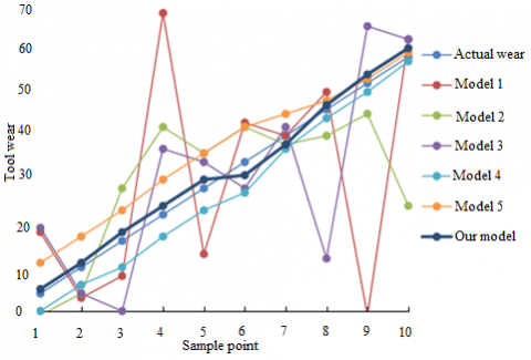
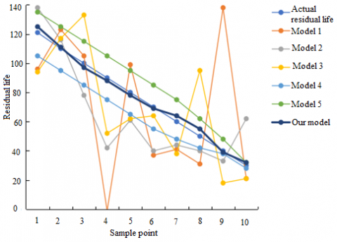
After the identification of tool wear features, 10 sets of data were randomly extracted as the test sets for verifying the accuracy of our model in predicting tool wear and residual life. The prediction performance of our model was compared with five models through comparative experiments. Figures 10 and 11 show the prediction results of all six models. The experimental results show that our model converged fast and had a small error in model training, and reduced the prediction error of tool wear and residual life to 7.1% and 8.5%, respectively. The series of improvement to the ELM effectively enhances the prediction precision of tool wear and residual life, making it possible to apply the prediction model to actual job processing.
Figure 10. Prediction results on tool wear
Figure 11. Prediction results on residual life
To provide a theoretical guide for improving the production techniques of hard alloy material cutting, this paper explores the detection of frictional wear for hard alloy tool material during high-speed cutting. Firstly, the theories on wave motion were cited to build a mathematical model for the frictional wear process of hard alloy tool material during high-speed cutting, and to analyze the wear mechanism. To weaken the interference of weakly important features, new strategies were developed to evaluate the feature importance, and recognize tool frictional wear, facing the high-dimensional small dataset on the monitoring signals of tool material wear. Through experiments, the results of Gini importance method and Lasso feature importance method were obtained, and residual analysis was carried out, confirming that the experimental data after feature selection are normal, and need no further screening. In addition, the trend of tool wear amount was tested at different cutting speeds and feed rates. The results demonstrate the feasibility of our algorithm in recognizing the hard alloy tool wear under high-speed cutting.
This research was funded by the Science and Technology Planning Project in Henan Province (Grant No.: 212102210326), the Key Research Projects of Henan Higher Schools (Grant No.: 21B460007) and Youth project of national scientific research project cultivation fund of Huanghuai University (Grant No.: XKPY-202104).
[1] Onyeme, C., Liyanage, K. (2021). A critical review of smart manufacturing and industry 4.0 maturity manufacturing & industry 4.0 maturity upstream industry. Advances in Transdisciplinary Engineering, Moving Integrated Product Development to Service Clouds in the Global Economy - Proceedings of the 21st ISPE Inc, International Conference on Concurrent Engineering, 15: 347-354.
[2] Guo, D., Li, M., Lyu, Z., Kang, K., Wu, W., Zhong, R.Y., Huang, G.Q. (2021). Synchroperation in industry 4.0 manufacturing. International Journal of Production Economics, 108171. https://doi.org/10.1016/j.ijpe.2021.108171
[3] Rai, R., Tiwari, M.K., Ivanov, D., Dolgui, A. (2021). Machine learning in manufacturing and industry 4.0 applications. International Journal of Production Research, 59(16): 4773-4778.
[4] Naitove, M.H. (2018). Digital manufacturing: Two medical molders embrace industry 4.0. Plastics Technology, 64(12): 38-42. https://doi.org/10.1007/978-3-319-25178-3_7
[5] Kamble, S.S., Gunasekaran, A., Sharma, R. (2018). Analysis of the driving and dependence power of barriers to adopt industry 4.0 in Indian manufacturing industry. Computers in Industry, 101: 107-119. https://doi.org/10.1016/j.compind.2018.06.004
[6] Wang, B., Liu, Z., Hou, X., Zhao, J. (2018). Influences of cutting speed and material mechanical properties on chip deformation and fracture during high-speed cutting of Inconel 718. Materials, 11(4): 461. https://doi.org/10.3390/ma11040461
[7] Zhang, X., Sui, H., Zhang, D., Jiang, X. (2018). An analytical transient cutting force model of high-speed ultrasonic vibration cutting. The International Journal of Advanced Manufacturing Technology, 95(9): 3929-3941. https://doi.org/10.1007/s00170-017-1499-z
[8] Dikshit, M.K., Puri, A.B., Maity, A. (2017). Analysis of rotational speed variations on cutting force coefficients in high-speed ball end milling. Journal of the Brazilian Society of Mechanical Sciences and Engineering, 39(9): 3529-3539. https://doi.org/10.1007/s40430-016-0673-9
[9] Ke, Q., Xu, D., Xiong, D. (2017). Cutting zone area and chip morphology in high-speed cutting of titanium alloy Ti-6Al-4V. Journal of Mechanical Science and Technology, 31(1): 309-316. https://doi.org/10.1007/s12206-016-1233-z
[10] Shi, Q., Pan, Y., Fu, X., Zhou, B., Zhang, Z. (2021). Effect of anisotropy and cutting speed on chip morphology of Ti-6Al-4V under high-speed cutting. The International Journal of Advanced Manufacturing Technology, 113(9): 2883-2894. https://doi.org/10.1007/s00170-021-06754-8
[11] Gobber, F.S., Fracchia, E., Rosso, M. (2019). Wear characterization of cemented carbide multipoint cutting tool machining AISI 4140 at high cutting speed: criteria for materials selection. In TMS 2019 148th Annual Meeting & Exhibition Supplemental Proceedings, 711-718. https://doi.org/10.1007/978-3-030-05861-6_69
[12] Zheng, G., Cheng, X., Li, L., Xu, R., Tian, Y. (2019). Experimental investigation of cutting force, surface roughness and tool wear in high-speed dry milling of AISI 4340 steel. Journal of Mechanical Science and Technology, 33(1): 341-349. https://doi.org/10.1007/s12206-018-1236-z
[13] Wang, Y., Su, H., Dai, J., Yang, S. (2019). A novel finite element method for the wear analysis of cemented carbide tool during high speed cutting Ti6Al4V process. The International Journal of Advanced Manufacturing Technology, 103(5): 2795-2807. https://doi.org/10.1007/s00170-019-03776-1
[14] Zheng, G., Xu, R., Cheng, X., Zhao, G., Li, L., Zhao, J. (2018). Effect of cutting parameters on wear behavior of coated tool and surface roughness in high-speed turning of 300M. Measurement, 125: 99-108. https://doi.org/10.1016/j.measurement.2018.04.078
[15] Kuram, E. (2018). The effect of monolayer TiCN-, AlTiN-, TiAlN-and two layers TiCN+ TiN-and AlTiN+ TiN-coated cutting tools on tool wear, cutting force, surface roughness and chip morphology during high-speed milling of Ti6Al4V titanium alloy. Proceedings of the Institution of Mechanical Engineers, Part B: Journal of Engineering Manufacture, 232(7): 1273-1286. https://doi.org/10.1177/0954405416666905
[16] Ming, W., Huang, X., Ji, M., Xu, J., Zou, F., Chen, M. (2021). Analysis of cutting responses of Sialon ceramic tools in high-speed milling of FGH96 superalloys. Ceramics International, 47(1): 149-156. https://doi.org/10.1016/j.ceramint.2020.08.118
[17] Chen, T., Qiu, C., Liu, X. (2017). Study on 3D topography of machined surface in high-speed hard cutting with PCBN tool. The International Journal of Advanced Manufacturing Technology, 91(5): 2125-2133. https://doi.org/10.1007/s00170-016-9940-2
[18] Wang, H., Yang, J., Sun, F. (2020). Cutting performances of MCD, SMCD, NCD and MCD/NCD coated tools in high-speed milling of hot bending graphite molds. Journal of Materials Processing Technology, 276: 116401. https://doi.org/10.1016/j.jmatprotec.2019.116401
[19] Sugihara, T., Takemura, S., Enomoto, T. (2016). Study on high-speed machining of Inconel 718 focusing on tool surface topography of CBN cutting tool. The International Journal of Advanced Manufacturing Technology, 87(1): 9-17. https://doi.org/10.1007/s00170-015-8006-1
[20] Zhu, Z.J., Sun, J., Lu, L.X. (2016). Research on the influence of tool wear on cutting performance in high-speed milling of difficult-to-cut materials. In Key Engineering Materials, 693: 1129-1134. https://doi.org/10.4028/www.scientific.net/KEM.693.1129
[21] Zou, B., Zhou, H., Huang, C., Xu, K., Wang, J. (2015). Tool damage and machined-surface quality using hot-pressed sintering Ti(C7N3)/WC/TaC cermet cutting inserts for high-speed turning stainless steels. The International Journal of Advanced Manufacturing Technology, 79(1-4): 197-210. https://doi.org/10.1007/s00170-015-6823-x
[22] Zhang, Y., Xu, X. (2021). Machine learning cutting force, surface roughness, and tool life in high-speed turning processes. Manufacturing Letters, 29: 84-89. https://doi.org/10.1016/j.mfglet.2021.07.005
[23] Meng, X., Lin, Y., Mi, S. (2021). The research of tool wear mechanism for high-speed milling ADC12 aluminum alloy considering the cutting force effect. Materials 2021, 14: 1054. https://doi.org/10.3390/ma14051054
[24] Chaus, A.S., Sitkevich, M.V., Pokorný, P., Sahul, M., Haršáni, M., Babincová, P. (2021). Wear resistance and cutting performance of high-speed steel ball nose end mills related to the initial state of tool surface. Wear, 472: 203711. https://doi.org/10.1016/j.wear.2021.203711
[25] Javidikia, M., Sadeghifar, M., Songmene, V., Jahazi, M. (2021). Low and high-speed orthogonal cutting of AA6061-T6 under dry and flood-coolant modes: Tool wear and residual stress measurements and predictions. Materials, 14(15): 4293. https://doi.org/10.3390/ma14154293
[26] Yasmin, F., Tamrin, K.F., Sheikh, N.A. (2021). Laser-assisted high-speed machining of aluminium alloy: The effect of ultrasonic-induced droplet vegetable-based cutting fluid on surface roughness and tool wear. Lasers in Engineering (Old City Publishing), 48(4): 195-225.