Hongjiang Cui | Shenghui Wu | Ying Guan*
© 2021 IIETA. This article is published by IIETA and is licensed under the CC BY 4.0 license (http://creativecommons.org/licenses/by/4.0/).
OPEN ACCESS
Through the improved delay-detached eddy simulation (IDDES), this paper establishes a 1:1 model for a high-speed train, and simulates the transient state of the train running 600km/h in a vacuum pipeline with the pressure of 1,000Pa. The results show that, following the Ω criteria, a pair of counterrotating vortexes can be captured, which alternatively shed near the tip of the last carriage, and propagate over a long distance along the flow direction. The motion and expansion of the vortexes are clearly three-dimensional (3D). Judging by the physical meaning of vortexes, the high vorticity vortexes mainly concentrate near the tip of the last carriage, while the low vorticity vortexes scatter across the wake zone. The latter vortexes have a low dissipation rate and are dominated by rotation. The turbulent energy and Reynolds stress of the wake field are very obvious near the tip of the last carriage, and attenuate quickly along the flow direction. This means the vortexes near the tip of the last carriage face a strong shear effect, and undergo apparent dissipation. Low turbulent energy and Reynolds stress are distributed in the downstream far from the tip of the last carriage, i.e., the interaction zone between vortexes and the ground / inner pipe wall.
vacuum pipeline, high-speed train, wake flow, vortex structure, turbulent performance
The rapid development of railways in China has contributed greatly to the economic growth and social advancement of the country. However, the increase in the speed of high-speed trains brings a series of problems, such as surging air resistance, wheel-rail adhesion, high operating noises, and the instability induced by snakelike motions. These problems severely bottleneck the speed increase of traditional high-speed trains [1, 2]. Once the train speed rises to 300km/h, the aerodynamic resistance of the dense air and the aerodynamic noise will have a great impact on the train [3]. The aerodynamic resistance is proportional to the square of the train speed, and the aerodynamic noise is proportional to the sixth power of the train speed. Neither of them is avoidable [4-7]. To further increase the train speed, the primary approach is to change the media density of the operating environment. For example, the operating resistance can be effectively reduced, if the train runs in a low-pressure closed pipeline.
The so-called vacuum pipeline is not completely vacuum. The high-speed train operating in such a pipeline will face the tunnel effect, which complicates the aerodynamic features of the operation, as well as the turbulent flow in the wake area of the train. Studies have shown that the tunnel effect on high-speed trains can be alleviated by improving the airtightness of the train and streamlining the shape of train head [8-11]. Due to the dense wake vortexes and turbulent features, the wake zone becomes the main source of aerodynamic resistance and aerodynamic noise of the train [12]. Similar to the tendon in fluid motion [13], the vortex structure directly affects the wake flow, giving birth to important aerodynamic phenomena. Early studies mainly derive turbulent coherent structures with vortex scalar, and then identify the vorticity concentration area, i.e., the vortex core. But this approach does not apply to laminar flow [14]. Later studies have demonstrated that vortex should also satisfy generalized Galilean invariance, and defined classic rules like Q criteria and λ criteria [15, 16].
Many Chinese scholars have explored the flow field and aerodynamic resistance law of high-speed trains from the perspectives of the vacuum degree, blockage ratio, and cross-sectional area of the vacuum pipeline. Considering the effects of compressibility of vacuum pipeline, Liu et al. [17] simulates the influence of pipeline pressure, blockage ratio, and train speed over the aerodynamic resistance on the train, with the aid of three-dimensional (3D) steady-state compressible turbulence. Huang et al. [18] numerically simulated the influence law of the vacuum degree, cross-sectional area, and ambient temperature over the aerodynamic resistance on high-speed trains. However, there is little report on the wake vortex and its turbulent features of high-speed trains in vacuum pipelines, which may otherwise shed light on resistance and noise reduction of trains operating in vacuum pipelines.
This paper sets up a simplified model for CRH380CL high-speed train, and adopted the improved delay-detached eddy simulation (IDDES) to emulate the transient state of the high-speed train running at 600km/h in a vacuum pipeline with the pressure of 1,000Pa and blockage ratio of 0.36. The vortex structure in the wake field of the train in the vacuum pipeline was captured and discussed, according to the Ω vortex criteria and its physical meaning. The turbulent features of the vortex structure were explored by analyzing physical quantities of the wake field, such as turbulent energy and Reynolds stress.
2.1 Numerical model and boundary conditions
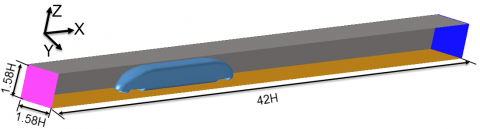
This paper establishes a 1:1 model of CRH 380CL high-speed electric multiple unit (EMU) train, and simplifies the EMU into the combination of the first carriage and the last carriage. The outer surface of the train was smoothened to ignore any protruding part. The bogie at the bottom of the train has a complex structure, which may induce complex flows. But this area has little to do with the vortex structure in the wake zone. Therefore, the bogie area was idealized in our model: The 1/4 fairing that covers the bogie was assumed to be perfectly connected with the sealing cover plate on the outer edge of train bottom, and the bogie structure was deleted, retaining only the parts near the head and tail of the train. The simplification does not change the aspect ratio, the streamline head and tail, the large height-to-length ratio, or the basic features of external flow field and wake turbulence during high-speed operation [19-21]. Figure 1 shows the simplified model of the high-speed train, where, H=3.8m is the height of the train. This parameter was taken as the characteristic length.
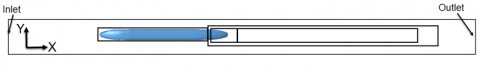
Drawing on the research of Liu et al. [12, 17, 22], the computational domain, i.e., the specific dimensions of the vacuum pipeline, was plotted as Figure 2. The pipeline is 42H in length, and 1.58H in width and height. The distance from the tip of the first carriage to the aur inlet is 9H. The distance from the tip of the last carriage to the air outlet is 20H. The bottom of the high-speed train is 0.15H above the ground. The blockage ratio is 0.36. As for the boundary conditions, the inlet was configured as a velocity boundary inlet, where is velocity is 600km/h in the positive direction of the x axis. The outlet was configured as a pressure outlet. The pipe walls were configured as slip walls. The ambient temperature and ambient pressure were set to 300K and 1,000Pa, respectively.
Figure 1. Simplified model for CRH380CL high-speed train
(a)
(b)
Figure 2. Dimensions of the pipeline for the high-speed train
2.2 Meshing
The head of the high-speed train has many complex surfaces. Thus, the train surface was discretized into triangular grids, and the flow field was meshed into nonstructured tetrahedron grids. In total, the boundaries of the train were emulated by 10 layers of grids. The grid thickness Dy in the first layer can be calculated by:
$\Delta y=\frac{\sqrt{80} L_{c} y^{+}}{\operatorname{Re}_{c}^{13 / 14}}$ (1)
where, Lc is the characteristic length; Rec is the Reynolds number corresponding to Lc.
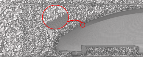
According to the relevant literature [23], the boundary grid thickness y+ of our model was set to 1. For the vacuum pipeline with the vacuum degree of 1,000Pa, the boundary thickness is about 0.00105H. As shown in Figure 3, the flow field was meshed into denser grids around the train, at the head of the last carriage, and in the wake zone. Three grid densification schemes were determined, namely, the coarse mesh (CM) scheme, medium mesh (MM) scheme, and ultrafine mesh (XM) scheme. The CM, MM, and XM schemes have 3,142,328, 4,203,577, and 10,299,676 grids, respectively.
Figure 3. Grid densification and enlarged view of densified areas
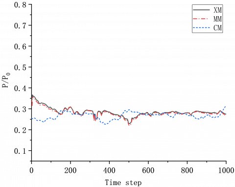
Figure 4. Curves of monitored pressure near the head of the last carriage during the 1,000 time steps
Grid independence was tested for the above three schemes. Through detached eddy simulation (DES), the wake zone monitoring results of the three schemes were compared after 1,000 time steps. Figure 4 shows the curves of monitored pressure near the head of the last carriage during the 1,000 time steps. It can be observed that the results of MM scheme agree well with those of XM scheme. The pressure trends of the two schemes are basically consistent. In the first 200 time steps, the pressure curve of the CM scheme deviated from that of the other two schemes. After the 200th time step, the pressure curve of the CM scheme gradually approached that of the other schemes, and the deviation became very small. After thorough consideration, the MM scheme was selected for grid densification. Finally, the computational scheme for vortex structure simulation of the high-speed train in vacuum pipelines was determined: the computational domain was meshed into 4,203,577 grids of the size between 0.02H and 0.08H.
2.3 Numerical scheme
According to Newton’s formula for shear stress of viscous fluids, the Navier-Stokes (N-S) equations can be derived to illustrate the motions of incompressible and compressible vicious fluids, based on the laws of the conservation of mass and momentum, respectively. Specifically, the N-S equation for compressible Newtonian fluids $\tau=\mu\left(\nabla U+\nabla U^{T}\right)-\frac{2}{3} \mu(\nabla \cdot U) I-\frac{2}{3} \rho k I$ can be expressed as:
$\begin{align} & \frac{\partial \rho U}{\partial t}+\nabla \cdot \left( \rho UU \right)= \\ & -\nabla p+\nabla \cdot \left( \mu \left( \nabla U+\nabla {{U}^{\text{T}}} \right)-\frac{2}{3}\mu \left( \nabla \cdot U \right)I-\frac{2}{3}\rho kI \right) \\\end{align}$ (2)
where, U is the velocity vector; ρ is density; p is the force acting on fluid microbodies; μ is dynamic viscosity; $\nabla U^{\mathrm{T}}$ cannot be simplified because $\nabla U^{T} \neq 0$ for compressible fluids.
N-S equations are the foundation of many algorithms, such as the large eddy simulation (LES) and Reynolds-averaged Navier-Stokes (RANS) model.
The IDDES model was adopted for simulation. This model combines the merits of LES and RANS, and supports the grid conversion between LES and RANS:
${{L}_{DES}}={{\tilde{f}}_{d}}\left( 1+{{f}_{e}} \right){{L}_{t}}+(1-{{\tilde{f}}_{d}}){{C}_{DES}}{{L}_{g}}$ (3)
${{\tilde{f}}_{d}}=\max \left( \left( 1-{{f}_{d}} \right),{{f}_{B}} \right)$ (4)
where, $\tilde{f}_{d}$ is the conversion function; fd is the conversion function of DDES model; fB is the conversion function of wall-modeled LES (WMLES); fe is the governing function of wall simulation:
${{f}_{e}}=\max \left( \left( {{f}_{e1}}-1 \right),0 \right){{f}_{e2}}$ (5)
During grid size calculation, the influence of wall distance was taken into account:
${{L}_{g}}=\min \left( \max \left( {{C}_{w}}{{d}_{w}},{{C}_{w}}{{h}_{\max }},{{h}_{wn}} \right),{{h}_{\max }} \right)$ (6)
where, $h \max (\Delta x, \Delta y, \Delta z)_{\max }$; hwn is the step length of grids in the vertical direction of the wall; Cw is a coefficient normally set to 0.15 in the IDDES model [24].
The Mach number was obtained as 0.49 by:
$Ma=\frac{v}{c}$ (7)
where, v is the velocity at a point in the flow field; c is the local sound velocity. The fluid was simulated with the ideal compressible gas model. For solver setting, the pressure-velocity coupling was introduced with Green-Gauss cell-based gradient method to compute the transient state of the governing function. The second-order implicit scheme was selected for the discretization precision of pressure and time. The model can solve 3D non-steady state turbulent flow.
The time step directly bears on the computing precision and stability. To ensure the stability of computing, the Courant number Co must be smaller than 1 [23]:
$\text{Co}=\frac{{{\text{U}}_{\infty }}\Delta \text{t}}{\Delta x}$ (8)
where, Dx is the grid spacing in the x direction; Dt is time step, which is calculated as 0.000458s.
2.4 Verification of model accuracy
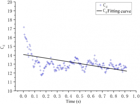
Figure 5. Scatterplot of the aerodynamic resistance coefficient Cd within 1s
Following the MM scheme, and the above boundary conditions, this paper computes the aerodynamic resistance and other parameters of the high-speed train running in the vacuum pipeline. Figure 5 presents the scatterplot of the aerodynamic resistance coefficient Cd within 1s. In most cases, the coefficient was near the straight line with the intercept of 14.079 and the slope of -2.039. After 0.1s, the coefficient fluctuated regularly with an average of 13.144. More than 80% of Cd values fell between 12.1 and 13.7. The result is very close to the conclusion of Liu et al. [12, 18]: the Cd value was 12.08 for a high-speed train running at 600km/h in a vacuum pipeline of the pressure 1,013.25Pa. The error between the two results was within 0.016% and 8%. This means our simulation model outputs reasonable and credible information about the wake field of the high-speed train in the vacuum pipeline.
The aerodynamic resistance coefficient Cd can be calculated by:
$F=\frac{1}{2}{{C}_{d}}\cdot \rho \cdot S\cdot {{u}^{2}}$ (9)
where, ρ is the air density; S is the wind area of the train; u is the relative velocity between the train and the air. According to the non-steady state simulation of the high-speed train, the aerodynamic resistance coefficient Cd was distributed like a pulse over time. The pulsation frequency is related to the vortex shedding at the tail of the high-speed train. Every wake vortex shedding causes a change to the aerodynamic resistance of the train [22].
3.1 Identification of wake field vortexes
The vortexes in the wake field of the high-speed train were captured by the Ω vortex identification method proposed by Liu et al. The vorticity was divided into a rotation part and a non-rotation part [14, 25]:
$\Omega =\frac{\left\| \mathbf{B} \right\|_{\text{F}}^{2}}{\left\| \mathbf{A} \right\|_{\text{F}}^{2}+\left\| \mathbf{B} \right\|_{\text{F}}^{2}+\text{ }\!\!\varepsilon\!\!\text{ }}$ (10)
where, $\varepsilon$ is an infinitesimal positive; A and B are the symmetric and antisymmetric tensors of velocity gradient, respectively; $\Omega \in[0, \quad 1]$ is a non-dimensional number representing the vorticity concentration, i.e., the proportion of rotating vorticity in total vorticity. If Ω=1, the fluid rotates like a rigid body. Thus, the vortexes are usually identified with Ω>0.5.
$\text{A=}\frac{1}{2}\left( \frac{\partial {{u}_{i}}}{\partial {{x}_{j}}}+\frac{\partial {{u}_{j}}}{\partial {{x}_{i}}} \right)$ (11)
$\text{B=}\frac{1}{2}\left( \frac{\partial {{u}_{i}}}{\partial {{x}_{j}}}-\frac{\partial {{u}_{j}}}{\partial {{x}_{i}}} \right)$ (12)
where, u is the vector velocity; i, j=x, y, z, i.e., the three directions of the three directions of vector velocity decomposition.
(a) Enlarged view of local vortexes near the last carriage
(b) Top view of wake field vortexes with Ω=0.52
Figure 6. Wake field vortexes
Figure 6 displays the wake field vortexes of the high-speed train in the vacuum pipeline, which are captured by the Ω vortex identification method. At the tip of the last carriage, two columns of counterrotating vortex pairs appeared, which were centrosymmetric along the span direction of the train. The symmetry was pretty obvious near the tip of the last carriage. The vortexes gradually expanded as they propagated away from the last carriage to the downstream. The expansion, coupled with the restriction by the inner wall of the pipeline, suppressed the centrosymmetric feature. After shedding from the tip of the last carriage, the vortex pairs moved to the outside of the span direction and to the ground in the area near the tip of the last carriage. After about x=2H, the vortexes propagated to the upper wall of the pipeline, while spiraling to the downstream. After hitting the inner wall, the vortex pairs quickly fragmented, expanded, and flattened. Therefore, the presence of the pipeline has a major impact on the shape and motion of the vortex structure.
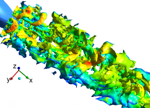
Figure 7 shows the wake field vortexes captured with different Ω thresholds. As the threshold increased from 0.52 to 0.85, the big vortexes in the wake field of the high-speed train always propagated for a long distance in the flow direction. The small vortexes far from the tail could also be captured. As mentioned before, the value of Ω represents the ratio of rotating vorticity to total vorticity. Therefore, the high vorticity area at the tip of the tail corresponds to a strong shear. The increase of Ω value indicates that the shear effect in the wake field weakens; the rotating vorticity accounts for a greater portion, and gradually dominates the wake field. As the threshold increased, the fragmented and flattened vortexes at the inner wall of the pipeline slowly disappeared. This means the vorticity and intensity of vortexes attenuate quickly after the vortexes hit the inner pipe wall. Dense vortexes could be observed in the vacuum pipeline. The vortex development in the wake field was obviously three-dimensional.
(a) Ω=0.52
(b) Ω=0.75
(c) Ω=0.85
Figure 7. Wake field vortexes at different thresholds
3.2 Turbulent energy
Turbulent energy measures the intensity of turbulence:
$\text{E=}\frac{1}{2}\left( \overline{{u}'{u}'}+\overline{{v}'{v}'}+\overline{{w}'{w}'} \right)$ (13)
where, u’, v’, and w’ are the pulsation velocities in the flow direction, span direction, and vertical direction, respectively.
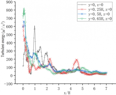
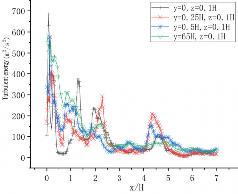
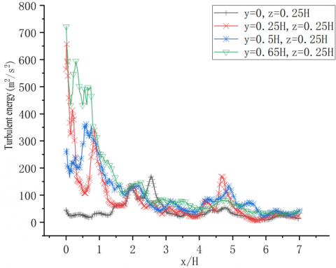
Figure 8 shows the time-averaged trends of turbulent energy in the wake zone. Note that x, y, z=(0,0,0) is the tip position of the last carriage. In the flow direction, the turbulent energy changed significantly at all positions in the span direction of the z=0 plane at the tip of the last carriage, when the distance was within x<3H from the tip of the last carriage; the turbulent energy changed relatively gently, when the distance was x>3H. The most prominent turbulent energy existed on the outside in the span direction. During the vortex development in the flow direction, turbulent energy peaks at other positions in the span direction appeared successively. After multiple oscillations, the turbulent energy quickly attenuated in the area of x<3H. At the center of the span direction y=0, the turbulent energy changed very violently as z changed from 0 to 0.1H, under the effect of bogie area vortexes at the bottom of the train. However, after z surpassed 0.25H, the turbulent energy became very small at the center of the span direction y=0. The trend of turbulent energy in the span direction is closely related to the span direction movement of vortexes. Near the tip of the last carriage, the vortexes carry a huge amount of turbulent energy. As the vortexes propagate to the downstream along the flow, their turbulent energy gradually dissipates. Besides, the span direction movement of the vortex structure leads to heterogenous distribution of turbulent energy in this direction. In addition, the turbulent energy is relatively large near the outer pipe wall, in the presence of the vacuum pipeline.
(a) z=0
(b) z=0.1H
(c) z=0.25H
Figure 8. Time-averaged variation of turbulent energy in the wake zone along the flow direction
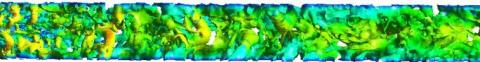
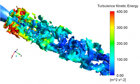
Figure 9 shows the vortex structure in the upstream and downstream of the wake field, which is identified by turbulent energy. The vortexes shedding near the tip of the last carriage had a high turbulent energy. The turbulent energy quickly attenuated as the vortexes propagated to the downstream. High turbulent energy was observed in vortexes on the outside in the span direction, and in the upper section in the vertical direction. All these areas witness the interaction between vortexes and the pipeline. That is, the vortexes are flattened and fragmented in these areas. Therefore, vortex deformation and fragmentation are accompanied by violent changes of turbulent energy.
(a) Upstream of wake field (Ω=0.6)
(b) Downstream of wake field (Ω=0.6)
Figure 9. Vortex structure identified by turbulent energy
3.3 Reynolds stress
Reynolds shear stresses $-\rho \overline{u^{\prime} v^{\prime}}$ and $-\rho \overline{u^{\prime} w^{\prime}}$ characterize the correlations between the components of pulsation velocity, and depend on the coupling between turbulent vortex structure and shear strain. In other words, Reynolds shear stress reflect the energy transmission between vortex flow and turbulent flow, and demonstrate the shear effect on vortexes.
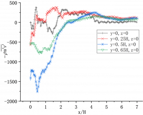
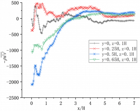
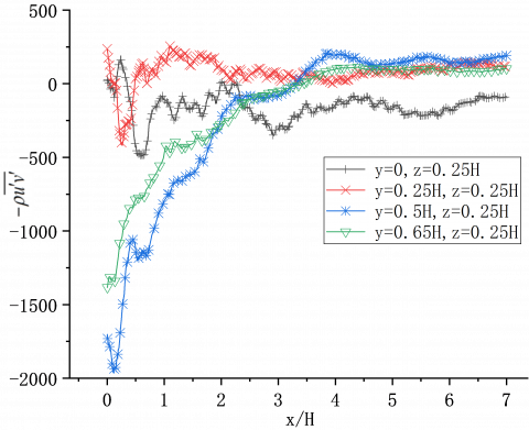
Figure 10 shows the time-averaged variation of the Reynolds stress $-\rho \overline{u^{\prime} v^{\prime}}$ along the flow direction at different vertical heights in the wake field of the high-speed train in the vacuum pipeline. Subgraph (a) presents the time-averaged variation of the Reynolds stress $-\rho \overline{u^{\prime} v^{\prime}}$ at z=0 (tip height) of the last carriage. It can be observed that the pulsation velocities u’ and v’ exhibited the closest correlations at y=0.5H, followed by y=0.65H in the span direction. This means the turbulent vortex is under a strong planar shear of x-y at y=0.5H near the tip of the last carriage. The shear effect exhibits as the shear deformation and motion of wake vortex structure along the span direction. With the growth of vertical height, the correlations between pulsation velocities u’ and v’ increased at y=0.65H in the span direction. Hence, the vortex also faces a strong planar shear of x-y at y=0.65H in the span direction. The Reynolds stress $-\rho \overline{u^{\prime} v^{\prime}}$ was the most prominent near the tip of the last carriage, and quickly attenuates in the area of x<3H. In the area of x>3H, the spanwise Reynolds stress $-\rho \overline{u^{\prime} v^{\prime}}$ basically oscillated about zero along the flow direction. However, the Reynolds stress was relatively large at y=0.5H on the outside of the span direction, far in the downstream of the tip of the last carriage along the flow direction. The Reynold stress fluctuations at y=0 and y=0.25H in the span direction were different from those at y=0.5H and y=0.65H on the outside of the span direction, indicating that these positions are affected by different shear flows.
(a) z=0
(b) z=0.1H
(c) z=0.25H
Figure 10. Reynolds stress $-\rho \overline{u^{\prime} v^{\prime}}$ curves along the flow direction
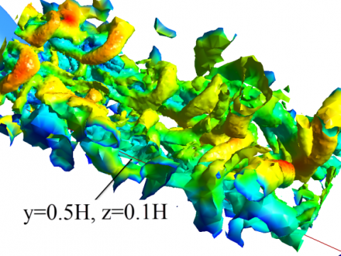
Figure 11 shows the vortexes in the area of 0<x<3H from the tip of the last carriage. In subgraph (a), the solid red line indicates the position of z=0 in the vertical direction and y=0.5H in the span direction from the tip of the last carriage. This position witnessed a clear transition from vortex expansion to shear deformation. In fact, this is where the Reynolds number $-\rho \overline{u^{\prime} v^{\prime}}$ underwent significant changes. In subgraph (b), the red circle corresponds to the y=0 position in the span direction near the tip of the last carriage. Under the effect of the bottom bogie area, this area saw the emergence of small vortexes moving upwards in the vertical direction. That is, the shear effect on vortexes corresponds to the trend of spanwise Reynolds stress at the position.
(a)
(b)
Figure 11. Vortexes near the tip of the last carriage
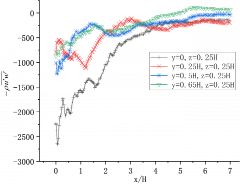
Figure 12 shows the time-averaged variation of the Reynolds stress $-\rho \overline{u^{\prime} w^{\prime}}$ along the flow direction at different vertical heights. Near the tip area, the pulsation velocities u’ and w’ were strongly correlated at y=0 and y=0.5H. However, the Reynolds stresses at the two positions had different signs, because the two positions are affected by different separated shear flows. Besides, with the growth of vertical height, the Reynolds stress was very large at y=0, while that at y=0.5H gradually decreased. This means the center of the train in the span direction is subjected to a strong planar shear of x-z. At the position of y=0.5H, the shear flow effect varied between z=0.25H, z=0.1H, and z=0, suggesting that different vertical heights are influenced by different vortexes. Specifically, near z=0.25H, the vortexes near the tip of the last carriage were mainly the two columns of counterrotating vortex pairs shedding along the head of the last carriage; the shear deformation along the vertical direction is the spiral expansion to the outside of the span direction and the upper part of the vertical direction. At z=0, and z=0.1H (i.e., near the tip of the last carriage), the main vortexes were the small vortexes shedding from the bottom bogie, which expand along the vertical direction. The Reynolds stress reflects the shear effect and deformation trend of vortexes. In the area of x>3H, the Reynolds stress $-\rho \overline{u^{\prime} w^{\prime}}$ on the outside of the span direction was larger than that at other positions in the span direction, a sign of the weak shear effect of the vortexes near the outer pipe wall in the downstream of the wake field. After expanding to the pipe wall, the flattening, expansion, and fragmentation of vortexes are all affected by the shear effect. The interaction between vortexes and inner pipe wall is an important mechanism that maintains local flow [23, 26].
(a) z=0
(b) z=0.1H
(c) z=0.25H
Figure 12. Reynolds stress $-\rho \overline{u^{\prime} w^{\prime}}$ curves along the flow direction
(1) By the Ω vortex identification method, this paper captures the wake field vortexes of a high-speed train running in a vacuum pipeline. Two columns of counterrotating vortex pairs are found shedding from the two sides of the tip of the last carriage, and moving to the downstream of the wake field along the flow direction. The movement is accompanied by the trends in the vertical and span directions. Judging by the physical meaning of vortexes, the high vorticity vortexes mainly concentrate near the tip of the last carriage, while the low vorticity vortexes scatter across the wake zone. With a low dissipation rate, the latter vortexes, dominated by rotation, can exist stably, and propagate over a long distance to the downstream of the wake field. The wake vortexes move along the flow direction. Once the vortex core reaches the side, upper, and lower walls of the pipeline, the interaction between vortexes and pipe wall will flatten and fragment the vortexes. The interaction is an important mechanism for vortexes to acquire energy from weak shear.
(2) According to the turbulent energy analysis on the wake field of the high-speed train in the vacuum field, the turbulent vortexes near the tip of the last carriage have a huge turbulent energy. As the vortexes develop to the downstream along the flow direction, the turbulent energy dissipates quickly in the area of 0<x<3H. Due to the spanwise motion of vortexes, the turbulent energy distribution is heterogenous in the span direction. In the area of x>3H, the interaction between vortexes and the ground / inner pipe wall makes the turbulent energy distribution more significant near the pipe wall and the ground.
(3) According to the Reynolds stress analysis on the wake field of the high-speed train in the vacuum field, the Reynold stress is very significant near the tip of the last carriage, and attenuates quickly in the area of 0<x<3H along the flow direction. The relatively high Reynolds stress reflects the strong shear effect on the vortexes. A low Reynolds stress, mainly near the outside of the span direction, exists in the downstream far from the tip of the last carriage. This means the vortexes face a weak shear effect near the pipe wall. In addition, the change trend of Reynolds stress demonstrates the deformation and motion of wake vortex structure, and, to a certain extent, manifests the energy transmission between turbulent vortexes and shear.
This work was supported by the Science Research Planning of Liaoning Provincial Education Department (Grant No.: LJKZ0509).
[1] He, S. (2010). The third wave of world railway development. China Report, 2010(12): 46-47.
[2] Shen, Z.Y. (2005). On developing high-speed evacuated tube transportation in China. Journal of Southwest Jiaotong University, 40(2): 133-137. https://doi.org/10.3969/j.issn.0258-2724.2005.02.001
[3] Feng, Z.W., Fang, X., Li, H.M., Cheng, A.J., Pan, Y.J. (2018). Technological development of high speed maglev system based on low vacuum pipeline. Engineering Science, 20(06): 105-111. https://doi.org/10.15302/J-SSCAE-2018.06.017
[4] Standard Policy and Strategy Committee. EN 14067-2: 2003 Railway application-Aerodynamics-Part 2: Aerodynamics on open track. Brussels: CEN, 2003.
[5] Standard Policy and Strategy Committee. EN 14067-3: 2003 Railway application-Aerodynamics-Part 3: Aerodynamics in tunnels. Brussels: CEN, 2003.
[6] Lighthill, M.J. (1952). On sound generated aerodynamically I. General theory. Proceedings of the Royal Society of London. Series A. Mathematical and Physical Sciences, 211(1107): 564-587. https://doi.org/10.1098/rspa.1952.0060
[7] Talotte, C. (2000). Aerodynamic noise: A critical survey. Journal of Sound and Vibration, 231(3): 549-562. https://doi.org/10.1006/jsvi.1999.2544
[8] Baron, A., Mossi, M., Sibilla, S. (2001). The alleviation of the aerodynamic drag and wave effects of high-speed trains in very long tunnels. Journal of Wind Engineering and Industrial Aerodynamics, 89(5): 365-401. https://doi.org/10.1016/S0167-6105(00)00071-4
[9] Howe, M.S. (2004). On the design of a tunnel-entrance hood with multiple windows. Journal of Sound and Vibration, 273(1-2): 233-248. https://doi.org/10.1016/S0022-460X(03)00498-X
[10] Anthoine, J. (2009). Alleviation of pressure rise from a high-speed train entering a tunnel. AIAA Journal, 47(9): 2132-2142. https://doi.org/10.2514/1.41109
[11] Murray, P.R., Howe, M.S. (2010). Influence of hood geometry on the compression wave generated by a high-speed train. Journal of Sound and Vibration, 329(14): 2915-2927. https://doi.org/10.1016/j.jsv.2010.01.036
[12] Liu, J.L., Zhang, J.Y., Zhang, W.H. (2013). Analysis of aerodynamic characteristics of high-speed trains in the evacuated tube. Journal of Mechanical Engineering, 49(22): 137-143. https://doi.org/10.3901/JME.2013.22.137
[13] Küchemann, D. (1965). Report on the IUTAM symposium on concentrated vortex motions in fluids. Journal of Fluid Mechanics, 21(1): 1-20. https://doi.org/10.1017/S0022112065000010
[14] Liu, C., Wang, Y., Yang, Y., Duan, Z. (2016). New omega vortex identification method. Science China Physics, Mechanics & Astronomy, 59(8): 1-9. https://doi.org/10.1007/s11433-016-0022-6
[15] JCR, H., Wray, A., Moin, P. (1988). Eddies, stream, and convergence zones in turbulent flows. Studying Turbulence Using Numerical Simulation Databases-I1, 193-208.
[16] Jeong, J., Hussain, F. (1995). On the identification of a vortex. Journal of Fluid Mechanics, 285: 69-94. https://doi.org/10.1017/S0022112095000462
[17] Liu, J.L., Zhang, J.Y., Zhang, W.H. (2014). The aerodynamic resistance and system parameter design of vacuum pipeline high-speed train. Journal of Vacuum Science and Technology, 34(1): 10-15.
[18] Huang, Z.D., Liang, X.F., Chang, N. (2019). Numerical analysis of train aerodynamic drag of vacuum tube traffic. Journal of Mechanical Engineering, 55(8): 165-172. https://doi.org/10.3901/JME.2019.08.165
[19] Bell, J.R., Burton, D., Thompson, M.C., Herbst, A.H., Sheridan, J. (2017). The effect of tail geometry on the slipstream and unsteady wake structure of high-speed trains. Experimental Thermal and Fluid Science, 83: 215-230. https://doi.org/10.1016/j.expthermflusci.2017.01.014
[20] Wang, J., Minelli, G., Dong, T., Chen, G., Krajnović, S. (2019). The effect of bogie fairings on the slipstream and wake flow of a high-speed train. An IDDES study. Journal of Wind Engineering and Industrial Aerodynamics, 191: 183-202. https://doi.org/10.1016/j.jweia.2019.06.010
[21] Hemida, H., Baker, C. (2010). Large-eddy simulation of the flow around a freight wagon subjected to a crosswind. Computers & Fluids, 39(10): 1944-1956. https://doi.org/10.1016/j.compfluid.2010.06.026
[22] Pan, Y.C., Yao, J.W., Liang, C., Li, C.F. (2017). Analysis on turbulence characteristics of vortex structure in near wake of high speed train. China Railway Science, 38(2): 83-88. https://doi.org/10.3969/j.issn.1001-4632.2017.02.13
[23] Pan, Y.C., Yao, J.W., Liu, C., Li, C.F. (2018). Discussion on the wake vortex structure of a high speed train by vortex identification methods. Chinese Journal of Theoretical and Applied Mechanics, 50(3): 667-676. https://doi.org/10.6052/0459-1879-17-383
[24] Wang, S.Y., Wang, G.X., Dong, Y., Deng, X.G. (2017). High-order detached-eddy simulation method based on a Reynolds-stress background model. Acta Physica Sinica, 66(18): 129-145. https://doi.org/10.7498/aps.66.184701
[25] Liu, C.Q. (2020). Liutex-third generation of vortex definition and identification methods. Acta Aerodynamica Sinica, 38(3): 413-431, 478. https://doi.org/10.7638/kqdlxxb-2020.0015
[26] Corjon, A., Poinsot, T. (1997). Behavior of wake vortices near ground. AIAA Journal, 35(5): 849-855. https://doi.org/10.2514/2.7457