Md Nuruzzaman | William Pao* | Faheem Ejaz | Hamdan Ya
© 2021 IIETA. This article is published by IIETA and is licensed under the CC BY 4.0 license (http://creativecommons.org/licenses/by/4.0/).
OPEN ACCESS
When hot and cold fluids flow through a converging T-junction, rapid temperature fluctuations occur in the mixing region due to the thermal mixing of fluids. This temperature fluctuation causes thermal fatigue, which is responsible for the shortening of service life in a T-junction. Hence, the design of T-junction for thermal mixing requires not only superior mixing performance but minimize thermal fluctuation during mixing is also desirable. The objective of the present paper is to determine the thermal mixing performance at the mixing region of T-junction with two different flow configurations. Water, at different inlet temperatures, is used as a working medium and is assumed incompressible. Two types of flow configurations, namely intersecting and colliding regular T-junction with a sidearm pointing at 12 o’clock position have been evaluated in this paper. Realizable k-epsilon turbulence model was assumed, and its validity benchmarked against RANS and RSM-EB turbulence models. The thermal mixing efficiency of both flow configurations is calculated and compared. The results show that the thermal mixing efficiency of both intersecting and colliding mixing tee increases with the increase of distance and time. Intersecting tee shows higher temperature fluctuation than colliding tee at the mixing outlet, but colliding tee shows higher thermal mixing efficiency than intersecting mixing tee.
T-junction, thermal mixing, mixing efficiency, turbulence model, temperature fluctuation
T-junction is a significant part of a piping network for combining and dividing the flow. Under certain favourable circumstances, it can be used for partial phase separation for multiphase flow [1]. T-junction is also a piping feature that is commonly seen in industries, e.g., for the cooling system in nuclear industry, LNG production/transportation, oil, and gas refining businesses [2].
In a combining or converging type T-junction for mixing, hot and cold fluids from two inlets combined at the mixing region and leave through the outlet a thermally well-mixed fluid. During the mixing, rapid temperature fluctuations occurred in the mixing region. This rapid temperature fluctuation can create high cyclic thermal stress and fatigue, eventually leading to the shortening service life of the T-joint. This reduction of the service durability of the pipeline may cause a catastrophic accident if not detected. Hence, in the design of thermal mixing using T-junction, it is desirable to have a mixing T-junction that is superior in thermal mixing performance that produces as little thermal fluctuation as possible.
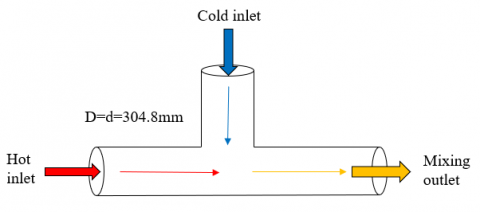
Recently, Malaysia Liquified Natural Gas (MLNG TIGA) of Bintulu, Malaysia has decided to refurbish their aging equipment. In one of the heat regenerative flow loops, they have decided to modify their thermal mixing T-junction by changing the flow configuration from a conventional intersecting T-junction as shown in Figure 1(a) to a colliding type T-junction, in Figure 1(b). The design in Figure 1(a) is called an intersecting mixing tee because the cold fluid is seen intervening in the flow path of the hot fluid in the main pipe. On the other hand, the design in Figure 1(b) is called colliding tee because the hot and cold fluid is seen colliding head-to-head with each other. One of the many questions that arise during the design is the thermal mixing efficiency of the new versus the old design. A careful literature survey shows that there is neither clear guideline nor rule-of-thumb practice to hint if the new design is better or worse than the old. This is the motive behind the present research.
(a)
(b)
Figure 1. The geometry of (a) intersecting and (b) colliding T-junction of MLNG plant
Thermal mixing of the same fluid is affected by numerous factors such as T-junction geometry, flow orientation, inclination angle, diameter ratio, inlet temperature difference, inlet fluid velocity, mass flow rate, fluid properties, flow types (turbulent or laminar flow), etc. To investigate different thermal mixing characteristics, many researchers have conducted a lot of experimental, numerical, and both studies by varying different influencing factors. Among these different influencing factors, hot and cold inlet temperature difference, inlet mass flow rate or velocity ratio are main key factors. Thermal mixing characteristics are mostly affected by these factors.
The inclination angle between the branch and main pipe plays an important role in thermal mixing. Thermal mixing is reached faster at a shorter mixing length for the inclination angles 45° and 60° and slower mixing is found at 30° or 90° [3]. In their experiment [3], 95% mixing was achieved at a distance of 3D (D is the main-pipe diameters) for an inclination angle of 45° and at a distance of 3.5D for an angle of 165° and a distance 4D for 60°angle. For 90° intersecting mixing tee, 95% mixing is achieved at the distance of 11D but for 90° colliding mixing tee, the distance required for 95% mixing is 5.5D. It is also observed that for 45° and 60° inclination angles, the mean temperature fluctuation dies away after 5D distance along the centerline of the mixing outlet. The influence of the jet angle on the turbulence fluids flow has been investigated by Hirota et al. [4]. It is found that the jet works most effectively with an angle of 45° against the main flow. Chuang and Ferng [5] found from their investigation that the mixing temperature is about uniform for 45° mixing tee for both downward injection (DI) and the horizontal injection (HI) but the temperature fluctuation is much greater for 90° mixing tee than 45° tee.
Inlet temperature difference of fluids or differential temperature is one of the most important factors which have a direct effect on thermal mixing. If the differential temperature is huge, it requires a longer duration and mixing length to achieve good thermal mixing. Consequently, it can be said that thermal mixing quality increases with the decrease of the inlet temperature difference and vice versa [6, 7]. Chen et al. [6] categorize mixing quality as good, medium, and bad if the temperature difference is less than 6℃, between 6℃ to 8℃ and more than 8℃, respectively. The mean temperature at the mixing region decreases and the thermal mixing increases with the increase of the distance of location along with the mixing outlet [8, 9]. The mean or normalized temperature can vary depending on the sampling location if the temperature is sampled at the position of the top (0°), bottom (180°), left (270°), right (90°), or at the center of the cross-section [10].
Branch and main pipe inlet mass flowrate ratio also plays an important role in thermal mixing. The flowrate ratio has a proportional relation with thermal mixing. If the flow rate ratio is higher, then the mixing quality will be higher and vice versa [11, 12]. The influence of branch and main pipe inlet flow rate ratio on thermal mixing quality has experimented in Chen et al. [6]. It was found that if the flowrate ratio is getter than 0.16 (Qb/Qm > 0.16), then the thermal mixing quality will be good. It was also found that mixing quality is medium and bad if the flow rate ratio is between 0.10 to 0.15 and less than 0.1, respectively.
Another influencing factor is the branch and main pipe velocity ratio which can affect thermal mixing, like flow rate ratio. In fact, the inlet mass flow rate is the alternative parameter of velocity. For conventional intersecting mixing tee, if the branch to main pipe inlet velocity ratio is higher, then reverse flow takes place which is responsible for better thermal mixing [13]. Inlet velocity ratio can also affect the mean temperature of the mixing fluid. It is found that if the branch and main pipe velocity ratio is higher, then the mean temperature at the mixing region will be lower [14]. From the work of Chen et al. [6], it is found that mixing quality is good, medium, and bad when the velocity ratio is more than 13.6, between 9 to 13.6, and less than 9, respectively.
Dewangan and Kumar [15] had performed a numerical study to observe the characteristics of fluid flow and heat transfer of incompressible fluids through a helical tube and they found that skim milk needs 4.5% more heat energy than apple sauce to achieve 60°C at the outlet to when the flow rate is 3L/min. Yang [16] had carried out a numerical simulation to investigate fluid flow features in a mechanical mixer and to numerically simulate the two-phase flow inside the cylinder of the mixer the Euler-Euler two fluids model was introduced. The thermal and hydrodynamic effect of Al2O3-water nanofluids which is considered as a non-isothermal laminar flow had been evaluated numerically by A. Mokhefi et al. [17]. Heat transfer performance of fluids in a rectangular channel has been investigated by Mirshafiee and Amiri [18] using internal obstacles and baffles. The result showed that triangular obstacles and elliptical baffles can produce higher heat transfer.
For numerical analysis using computational fluid dynamics (CFD) software, different turbulence models, such as LES, RANS, URANS, DES, k-ε, k-ω are used. Numerically, Large Eddy Simulation (LES) is preferred [19] because it could predict turbulent mixing with high accuracy and precision. Accompanying the high accuracy is an equally high computational cost and time. The Reynolds-Averaged Navier-Stokes (RANS) and Unsteady Reynolds-Averaged Navier-Stokes (URANS) turbulent models, which were less expensive than LES, were also highly recommended [20, 21]. Kang et al. [10] performed a transient numerical analysis for the Vattenfall T-junction test by using Detached Eddy Simulation (DES) turbulence model. They evaluated the applicability of the DES turbulent model for turbulent thermal mixing by comparing the numerical results with experimental data. To visualize the temperature fluctuation in T-junction, temperature measurement experiments in a pipe wall [22] and temperature distribution visualization experiments [23] have been conducted using FATHER and FATHERINO facilities. The temperature distribution was calculated by Kuhn et al. [24] using CFD code to compare temperature which had been measured by infrared rays via a thin brass pipe in FATHERINO. The effect of modelling on temperature fluctuation had been investigated by Howard and Pasutto [25] using code Saturne and some models such as LES Dynamic, LES Smagorinsky, and WALE.
In this research, the thermal mixing performance of hot and cold fluid mixing in intersecting and colliding type converging T-junctions has been investigated numerically by assuming incompressibility of fluid and realizable k-ε turbulence model. This k-ε turbulence model with two equations is widely used in industrial applications [26, 27]. This K-ε model is proved to produce satisfactory results [3] This model was selected due to a good performance in flows which possesses strong gradients in temperature or pressure, separation, and recirculation due to turbulence [28]. The assumed turbulence model has been validated with RANS and RSM-EB turbulence models in the open literature. Temperature fluctuations, and thus its efficiency, at different locations of the mixing region, have been investigated at different temporal and spatial locations.
In the following, governing equations mimicking the phenomenon of thermal mixing in a T-junction are briefly discussed. They comprised of the continuity equation related to the pressure, three momentum equations related to the fluid velocities, energy equation related to the temperature variation, k-ε models related to the kinetic and dissipation energies. The flow is assumed incompressible since the medium is water and the range of velocities is modest.
2.1 Continuity
The continuity equation is also referred to as the conservation of mass. According to the continuity equation, the total amount of fluids entering through the inlet is equal to the sum of fluid leaving through the outlet and the accumulation of fluid in the control volume. The continuity equation can be written as,
$\frac{\partial \rho}{\partial t}+\nabla \cdot(\rho u)=0$ (1)
where ‘ρ’ is the density of the fluid and ‘u’ is the velocity vector.
2.2 Momentum
Momentum equations are also referred to as Navier-Stokes equations. Momentum equations are used for the conservation of momentum at the inlet and outlet of fluid flow through pipelines. The momentum equation for gas is given below:
$\frac{\partial}{\partial t}(\rho u) \nabla \cdot(\rho u \otimes u)=-\nabla \mathrm{p}+\nabla \cdot \tau+\rho \mathrm{g}$ (2)
where ‘p’ is the pressure, $\tau$ is the 2nd-order deviatoric stress tensor, and ‘g’ is the gravity acceleration vector.
2.3 Energy
The conservation of energy can be written as,
$\rho C_{p}\left[\frac{\partial T}{\partial t}+(u . \nabla) t\right]=K \nabla^{2} T+\emptyset$ (3)
where ‘Cp’ is the specific heat at constant pressure, ‘k’ is the thermal conductivity of the working fluid, Φ is the dissipation function representing the work done against viscous forces, which is irreversibly converted into internal energy. It is defined as:
$\emptyset=(\tau . \nabla) u$ (4)
For a more in-depth discussion about the Navier-Stokes equations, the readers could refer to the study [29] for explanation and it would not be further elaborated here.
In this study, ANSYS FLUENT 2020R1 had been chosen for fluid dynamics simulation of thermal mixing in T-junctions. It was considered as state-of-the-art CFD software for numerical investigation of fluid flow problems, and also for heat transfer in different complex geometries [30]. FLUENT had different turbulent models for both single-phase and multiphase flow. The subject of turbulent flow is extremely complex and difficult. To summarize, turbulent flows were classified by the length and time scales of eddies. The large eddies could be solved directly, and the small eddies were modelled with the Large Eddies Simulation model which is time dependent. The entire continuum of turbulent scales can be resolved directly using a method called Direct Numerical Simulation (DNS). Even though the high accuracy and precision of these models were desirable, it is not always practical due to cost and time constrain.
The k-ε model is a commonly used turbulence model to describe the characteristics of turbulent flows. This model was first proposed by Kolmogorov in 1942, then modified by Tennekes and Lumley [31]. Standard, RNG and Realizable k-ε models are some other variants of the k-ε model. In general, the k-ε model relied on two transport variables, namely the transported kinetic energy and dissipation, to represent the effects of convection and diffusion of turbulent energy. In the present study, the realizable k-ε model was adopted for simulation due to its short turnover time and ease of deployment.
3.1 Solution procedure and mesh dependency test
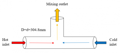
The numerical simulation consisted of three main steps: namely pre-processing, solution procedures, and post-processing. The pre-processing included geometry modelling, mesh generation, boundaries/surfaces definition, mesh independence test, etc. Normalized temperature at mixing region is used as the ultimate criterion for mesh convergence test. If the mesh is convergent, it will go to the next step. If the mesh is not convergent, then it will return to mesh generation step for mesh improvement to generate a fine mesh. The solution procedure included selecting the appropriate CFD model, material, prescribing boundary conditions, solver, etc. In post-processing, calculated numerical solutions were extracted and subjected to further manipulation to obtain the desired outcome. A brief flowchart for the entire CFD numerical procedure is shown in Figure 2.
Figure 2. Solution procedure of computational fluid dynamics
3.2 Geometry of T-junction
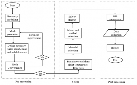
For the present paper, a simple T-junction geometry has been chosen. The main pipe and branch pipe diameter are assumed the same and the inclination angle between these two pipes is 90°. This T-junction is kept at a horizontal position so that the influence due to gravity can be minimized. Though it is connected to a long and complex piping system, only a small section is taken under consideration to reduce calculation time. The 3D design of the mixing tee and its parameters are shown in Figure 3.
Figure 3. Geometry and its different parameters
3.3 Mesh generation and mesh quality
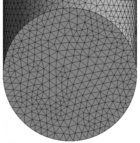
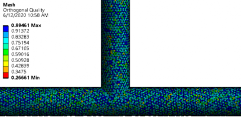
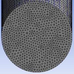
In this study, tetrahedral meshes were used as it is more economical and can decrease false diffusion more effectively than other types of meshing method [30]. Figure 4 showed the generated meshes at the side of the T-junction and the cross-sectional area of the outlet. Mesh skewness and orthogonal quality were performed for quality assurance purposes to ensure that the generated meshes were not overly distorted. The value ranges that indicate the skewness and orthogonal quality are listed in Table 1. For skewness quality lowest value provide excellent mesh quality. The skewness quality decreases gradually with the increase of number value. But orthogonal quality shows a proportional relation with the number value with is quite opposite relation with the skewness quality. The quality assurance of mesh was shown in Figure 5, showing very little distortion or unacceptable tessellation.
Figure 4. Side view and mixing outlet view of the generated mesh
Table 1. Mesh quality value range
|
Mesh quality |
Skewness quality |
Orthogonal quality |
|
Excellent |
0-0.25 |
0.98-1.00 |
|
Very good |
0.25-0.50 |
0.95-0.97 |
|
Good |
0.50-0.80 |
0.80-0.94 |
|
Acceptable |
0.80-0.94 |
0.50-0.80 |
|
Bad |
0.95-0.97 |
0.25-0.50 |
|
Unacceptable |
0.98-1.00 |
0-0.25 |
(a) Skewness quality
(b) Orthogonal quality
Figure 5. Mesh quality assurance check using skewness and orthogonality
3.4 Mesh convergence test
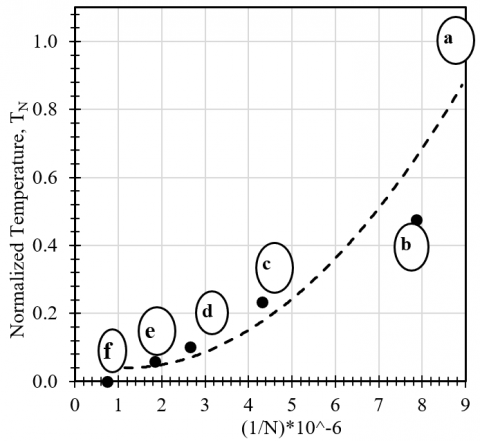
Mesh dependency test was an important step because it was an indirect way of quality assurance to ensure that the numerical problem was correctly possessed, and the discretization was consistent such that the solution was converging to numerical true solution as the total number of discretization increased. In this study, six different test cases were chosen to evaluate the sensitivity of output results on mesh size or element numbers. Figure 6 showed different mesh refinement in increasing order from left to right. The normalized temperature of the mixing outlet was chosen as convergence criteria and plotted along Y-axis. Along the X-axis, the value (1/N)x10-6 had been plotted where N is the total element number. Normalized temperature indicates the distribution of temperature along the mixing region of hot and cold fluids. It can be defined as [11],
$T^{*}=\frac{T-T_{c}}{T_{h}-T_{c}}$ (5)
where, T* is normalized temperature, T is instantaneous temperature, Tc and Th indicate cold and hot inlet temperature respectively. It was clear from Figure 7 that the normalized temperature decreased with the increase of total element numbers, indicating solution convergent to ‘true’ solution as the mesh was refined. With the increase of total mesh element number, the quality of mesh improves, and difference between two consecutive output temperatures decrease. As a result, the value of temperature distribution or normalized temperature decrease with the increase of total mesh element number. It was found from Figure 7 that the difference between normalized temperature was much higher between point ‘a’ and ‘b’, and somewhat fluctuating normalized temperature values. Hence, it can be concluded that mesh ‘a’ and ‘b’ were not acceptable. In fact, Figure 7 could be used directly to estimate the ‘error’ due to mesh discretization, e.g., in order to keep the ‘error’ below 10%, Figure 8 suggested only mesh ‘d’ and beyond should be used. In the present study, mesh ‘e’ with the total element of 540,347 was chosen for calculation. From here onwards, unless otherwise stated, the mesh size used for different case studies would always be referred to in Figure 8 as the norm.
a) Coarse mesh (112043)
b) Coarse mesh (127030)
c) Intermediate (231567)
d) Fine mesh (375870)
e) Fine mesh (540347)
Figure 6. Five levels of tessellation refinement for mesh sensitivity check
Figure 7. Mesh sensitivity test using realizable k-ε turbulence model
Figure 8. Schematic of the mixing-tee model for the work of Ming and Zhao
4.1 Model validation-1
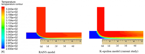
The model validation serves as an additional layer of quality assurance for the deployed methodology and adoption of the fit-for-purpose turbulent model. The first validation example was selected from Ming and Zhao [30]. In their paper, the RANS turbulence model was simulated with water as a working medium. The problem was an intersecting regular mixing tee, with the same diameter of the branch and main arm at 10 cm. The T-junction was positioned horizontally with the branch arm pointing at the 12 o’clock position. Coldwater entered the main arm with a velocity of 0.27 m/s at 20℃ while hot water entered through the branch arm with a velocity of 1.26 m/s at 53℃. The height of the branch arm was 50 cm, the entry distance for the cold water from the main arm is 50 cm. A simple hand calculation showed that the outlet temperature will reach 47℃. The schematic of the model problem by Ming and Zhao [30] is shown in Figure 8.
Figure 9 showed the comparison of the steady-state temperature contour of the RANS model [30] and the k-ε model by the present study. The results by Ming and Zhao [30] showed a better resolution of temperature segregation with a sharp boundary in between hot and cold water while the k-ε model showed a more dispersed and blurry temperature boundary. Both mixing outlets had a similar temperature of 320 K or 47℃ but the RANS model showed a slightly higher temperature.
Figure 9. Comparison of temperature contour of Ming and Zhao [30] and current study
Figure 10. Comparison of velocity contour of Ming and Zhao [30] and current study
Figure 10 shows the comparison of the magnitude of velocity contour between Ming and Zhao [30] RANS model and present simulation using the k-ε model. Again, it was noticed that [30] produced distinctive regions of velocities with very sharp and well-defined boundaries while the present model showed blurry velocity regions and boundaries. At both hot and cold inlets, velocities were uniform with no detectable significant gradient because of no mixing of flow streams. At the mixing junction, high velocities gradients were observed. At the main pipe outlet near the joint, the velocity is significantly lower as there is no fillet at the weld of the T-joint branch and main pipe. On the other hand, on the opposite side of the joint, at 0.5d to 3d distance of mixing outlet, the highest velocity was found as the hot and cold fluids intersected at 90° angle mostly in this region. So, from 0d to 4d distance at the outlet, three layers of the region for low, medium, and high velocity were found. But after 4d distance, the velocity becomes uniform as the mixing of two fluids of different velocities and temperatures took place. One more noticeable matter is that there is a low velocity at the region adjacent to the wall due to the viscous effect and adhesive force between fluids and structure. From Figure 10, a blue colour line can be observed that near the wall region which indicates a low velocity. During numerical set up, no slip boundary condition has been added. As a result, a friction force is acted at the contact surface between fluid and solid pipe and the velocity is reduced.
4.2 Model validation-2
The second model was chosen from the work of Santis and Shams [21]. In their study, the branch pipe diameter was 50 mm, while the main/run pipe was 150 mm, making the diameter ratio 0.33. Both cold and hot inlet has the same entry length of 3D, which is 450 mm. The hot fluid entered the main pipe with a velocity of 1.46 m/s at 48℃ while the cold fluid entered the branch pipe with a velocity of 1 m/s at 33℃. In this case study, the T-junction is laid horizontally, and the branch pipe is pointing at the 6 o’clock position, see the schematic diagram in Figure 11. Water is the working fluid. Because of the velocity difference, the mixing outlet will be dominated by the hot fluid, and the mixing has a temperature differential of 15℃, with a velocity ratio of 0.68. Simple hand calculation shows an outlet temperature of 47℃ or 320 K.
Figure 11. Geometry and its parameters for validation
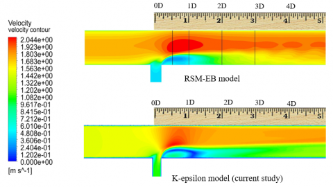
Santis and Shams [21] performed their simulation with Reynolds Stress Model (RSM-EB). Figure 12 shows the comparison of the temperature contour of [21] and the present k-ε model. Both results showed two regions of medium and high temperature at the mixing outlet with a clear distinctive static thermal layer at the upper part of the outlet tube. This indicated poor thermal mixing. Figure 13 showed that RSM and k-ε could produce comparable temperature results.
Figure 12. Comparison of temperature contour of [21] and current study
Figure 13. Comparison of velocity contour of Santis and Shams [21] and current study
Figure 13 is a comparison of the magnitude of velocity contour of the Ref. [21] with the RSM-EB model and the k-ε model of the current study. The RSM model showed a sharp velocity contour that looked like a turbulent wave while the k-ε model showed good similarity, its velocity contour was dispersed with lacked the turbulent detail.
Both validation studies concluded that the deployed CFD methodologies are correct, and the resulting temperature contour is comparable to published literature. There is a good similarity between the velocity contour but the k-ε model shows a noticeable lack of turbulence detail in exchange for faster turnover time.
4.3 Comparative study of thermal mixing between intersecting and colliding T-junction
Table 2. Parameters of T-junction geometry
|
Geometric parameter |
Dimension |
|
Diameter of the main pipe, D1, D2 |
304 mm/12 inches |
|
Diameter of the branch pipe, D3 |
304 mm/12 inches |
|
Total Length of the main pipe, L1 |
2000 mm |
|
Partial Lengths of two sides of the main pipe, L2, L3 |
1000 mm |
|
Length of branch pipe, L4 |
1000 mm |
The present study is a comparative study of thermal mixing of water of different temperatures inside intersecting and colliding mixing tees. The main pipe and branch pipe diameters are assumed the same, and the data related to this model are summarised in Table 2. Because the comparison is to observe the impact due to change in flow configuration, the same geometry and boundary conditions have been used in both models. The observation and temperature sampling location for both models is the mixing outlet.
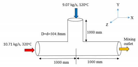
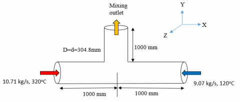
In a converging intersecting mixing tee, hot water enters through the main pipe inlet and cold water enters through the branch pipe inlet. Fluids from two inlets intersect at the right angle (90°) and a mixer of fluids leaves through another end of the main pipe. In colliding mixing tee, hot water enters through one end of the main pipe and cold gas through another end of the same pipe. Fluids from two inlets collude from the opposite directions (180°). Fluids after mixing leave through the branch pipe. For both mixing tees, the inlet temperature difference is 200℃, and the branch to main pipe mass flow rate ratio is 0.85. A No-slip boundary condition has been used at the wall of the T-junction. The flow configurations and boundary conditions for both mixing tees are shown in Figure 14.
(a)
(b)
Figure 14. boundary conditions and flow direction for (a) intersecting and (b) colliding T-junction
Figure 15. Temperature contour of (a) intersecting and (b) colliding mixing tee
Figure 15(a) shows the temperature contour of intersecting mixing tee, and three distinct regions of a high, medium, and low temperature are found. Even after 3d distance, a high-temperature difference is found, and thermal mixing just takes place in the middle of the mixing outlet. There is a clear hot stagnation layer that cannot be penetrated by the cold fluid. The temperature contour of colliding mixing tee is shown in Figure 15(b). At the branch pipe, which is considered here as a mixing outlet, three regions of temperature are found, similarly, to intersecting tee. Thermal mixing performance increases with the increase of mixing length.
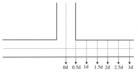
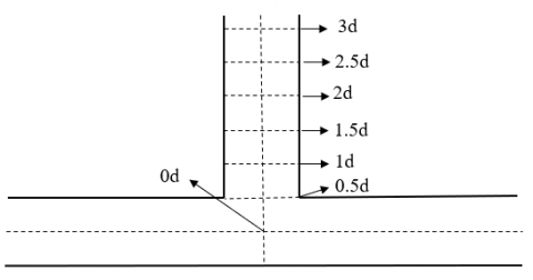
Figure 16 shows the sampling location of different cross-sectional planes at the mixing outlet for both T-junctions in terms of pipe diameter. All the planes are drawn at the outlet as the thermal mixing takes place in that region.
(a)
(b)
Figure 16. Location of different planes of the cross-section at mixing outlet for (a) intersecting and (b) colliding mixing tee
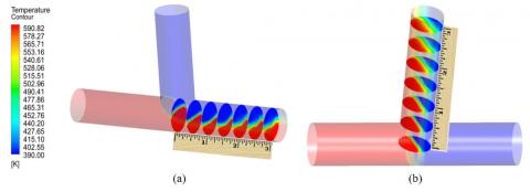
To observe a better one-to-one comparison, Figure 17 shows the cross-sectional view of temperature at different planes of mixing outlets. The scale attached with the mixing outlet of the T-junction indicates the distance of different cross-sections in terms of main pipe diameter (1, 2, 3 means 1d, 2d, 3d distance). As expected, thermal mixing quality for both T-junctions increases with the increase of distance, but the colliding tee is seen to perform slightly better than intersecting tee. At 0d, thermal mixing quality is low as hot and cold fluids just begin to meet at that point.
Figure 17. Temperature contour of the cross-section of (a) intersecting and (b) colliding mixing tee
Figure 18. Cross-sectional temperature contour at 3d distance of (a) intersecting and (b) colliding mixing tee at different time steps
Figure 19. Comparison of average temperature fluctuations between Colliding and Intersecting mixing tee
The thermal mixing process of fluids having higher temperature differences also depends on the time taken for mixing. In this study, a transient simulation of 10 seconds has been performed for more accurate analysis. Temperature variation after 10 seconds is neglected because there is no change in temperature profile after that. Figure 18 compares the cross-sectional temperature contours at the plane 3d distance from the mixing point for both intersecting and colliding mixing tee at different time steps. It is found there is little change in temperature contours for different time steps in both mixing tees. However, the colliding tee shows a significant and noticeable mixed layer in comparison to intersecting tee.
To analyse the data in detail, Figure 19 shows the average temperature fluctuation at different locations of mixing outlets for both intersecting and colliding mixing tee. The highest average temperature in intersecting T-junction is found at the plane of 0d distance as the thermal mixing is just started at this plane. From Figure 19, it is found that for intersecting mixing tee, the intensity of temperature fluctuation is much higher as it fluctuates from 472.5k to 547k and the fluctuation range is 74.5℃. This means intersecting mixing tee has lower thermal mixing quality as the temperature difference is high. But in colliding mixing tee, temperature fluctuation is much lower as it fluctuates between the temperature 501k to 507k, and the difference is only 6℃. This indicates that colliding mixing tee has higher thermal mixing performance than intersecting mixing tee.
In the transient simulation, the temperature at any point or plane at the mixing outlet changes with the change of time. The average temperature of the cross-section at different locations and for different time steps are shown in Figure 20. The average temperature fluctuates with time, and it is also dependent on location. In intersecting T-junction at 0d plane, the highest temperature is found for different time steps, and
it is lower after 0.5d distance. From Figure 20(a), the intensity of temperature fluctuation is very high from 0s to 4s. After 4 seconds, the fluctuation mellows down. Overall, for intersecting mixing tee, the temperature fluctuates from 472.5 K to 547 K and the maximum temperature difference at the mixing outlet is 74.5℃. The temperature behaviour in colliding mixing tee is completely different from intersecting tee. Initially, when mixing of different temperature fluid just started, the average temperature is 493 K for all planes at different locations. But the average temperature suddenly jumped to 505 K within 2 seconds and starts to plateau very quickly. In colliding mixing tee shown in Figure 20(b), the average temperature fluctuates from 493 K to 508 K and the maximum temperature difference at the mixing outlet from 0s to 8s is 15℃. It can be concluded that temperature fluctuation at the mixing outlet in colliding mixing tee is much lower than intersecting mixing tee. Consequently, the thermal mixing performance of colling tee is better than intersecting tee.
(a)
(b)
Figure 20. Temperature distribution at the different cross-section for different time steps for (a) intersecting and (b) colliding mixing tee
4.4 Calculation of thermal mixing efficiency
To find out thermal mixing performance of hot and cold fluids more accurately, it is required to calculate the Temperature Mixing Degree, TMD [32], defined as:
$T M D=1-\frac{\Delta T_{\max }}{\Delta T_{i n}}$ (6)
where, $\Delta T_{\max }$ is the maximum temperature difference at any desired cross-section and $\Delta T_{in }$ is the inlet temperature difference of hot and cold fluids. TMD is a dimensionless parameter that can be expressed by fraction or percentage. TMD = 1 indicates complete mixing or 100% thermal mixing efficiency when there is no temperature difference of fluids in the mixing regions. In that case, the temperature distribution is uniform, no fluctuation of temperature is found. TMD = 0 refers to no temperature mixing of the fluid. In this study, inlet fluid temperature difference is 200℃ and $\Delta T_{\max }$ is a variable that depends on the locations of different planes.
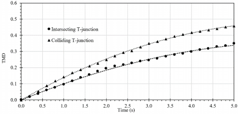
The relation between thermal mixing efficiency at different planes and the distance of those planes is shown in Figure 21 where “L” is mixing length and “d” is the diameter of the pipe. From Figure 21, it is apparent that for both intersecting and colliding mixing tee, TMD or thermal mixing efficiency increases with the increase of mixing length. From 0d to 1d, the efficiency increases by 20% for intersecting and 30% for colliding mixing tee. The rate of increase in TMD is much higher in this region. After 1d, the efficiency increases at about a uniform rate until 3d distance. At 3d plane, the thermal mixing rate is about 50% for colliding and 37% for intersecting T-junction. After 3d distance, an increase in efficiency is not significant. It can be observed that thermal mixing efficiency for both T-junctions is not very high in this study due to prescribed boundary conditions. From Figure 22, it is also noticeable that the thermal mixing efficiency of colliding mixing tee is consistently higher than intersecting T-junction.
Figure 21. Variation in TMD for intersecting and colliding mixing tees at various planes of different locations
Figure 22. Variation in TMD for intersecting and colliding mixing tees at 3d plane for different time steps
Variation of TMD or thermal mixing efficiency for colliding and intersecting mixing tee sampled at 3d distance at different time steps is shown in Figure 22. Here again, it is apparent that the TMD for a colliding tee is always consistently higher than intersecting tee at different timesteps. It is also found that TMD is time-dependent; it increases with the increase of time.
A numerical study has been carried out using CFD software to analyse thermal mixing in T-junctions with different flow configurations. One of the main concerns when analyzing thermal mixing was the incorporation of a good turbulent model. Even though LES and DNS are the highest recommended model in literature due to their accuracy, the accompanying high computational cost and time made them formidable. The present paper chooses to use a fit-for-purpose realizable k-ε turbulence model for this purpose. The numerical solution from this turbulent model is benchmarked with RANS and RSM-EB model for solution quality assurance. It was found that the k-Ԑ model produced comparable temperature contour but less satisfactory velocity contour, lacking the details of turbulence features.
To compare the thermal mixing performance and thermal fluctuation of mixing Tee with different flow configurations, a simple comparative test case was devised, using water as a working medium. Intersecting mixing tee was shown to have higher temperature fluctuation during mixing. Colliding mixing tee was shown to possesses better thermal performance when compared to intersecting tee.
The present study provides a clear idea and guideline for the selection of mixing T-junctions of similar nature. The present research has some limitations such as the effect of inclination angles between a branch and main pipe, diameter ratio, velocity ratio, inlet pressure, etc. are not analysed in this study.
The authors wish to acknowledge the research funding of Yayasan Universiti Teknologi PETRONAS under YUTP-015LC0-252 and Ministry of Higher Education Malaysia under Fundamental Research Grant Scheme FRGS/1/2019/TK03/UTP/02/10.
|
CFD |
Computational Fluid Dynamics |
|
Cp |
specific heat at constant pressure (Jkg-1 K-1) |
|
D |
diameter of main pipe (m) |
|
d |
diameter of branch pipe (m) |
|
g |
gravitational acceleration (ms-2) |
|
k |
Turbulent kinetic energy (J/kg = m2s-2) |
|
LES |
Large Eddy Simulation |
|
LNG |
Liquified Natural Gas |
|
MLNG |
Malaysia Liquified Natural Gas |
|
N |
Total number of mesh elements |
|
Q |
Mass flow rate (kgs-1) |
|
RANS |
Reynolds-Averaged Navier-Stokes |
|
RSM-EB |
Reynolds Stress Model-Elliptic Blending |
|
TMD |
Temperature Mixing Degree |
|
$\Delta T_{\max }$ |
maximum temperature difference at different plane (K) |
|
$\Delta T_{in }$ |
inlet temperature difference (K) |
|
URANS |
Unsteady Reynolds-Averaged Navier-Stokes |
|
Greek symbols |
|
|
$\varepsilon$ |
Turbulent kinetic energy dissipation rate (Jkg-1s-1 = m2s-3) |
|
$\omega$ |
specific dissipation (s-1) |
|
$\rho$ |
Density (kgm-3) |
|
$\tau$ |
2nd-order deviatoric stress tensor |
|
$\Phi$ |
dissipation function |
|
Subscripts |
|
|
b |
branch |
|
m |
main |
|
max |
maximum |
|
in |
inlet |
|
x |
Cartesian x coordinate |
|
y |
Cartesian y coordinate |
|
z |
Cartesian z coordinate |
[1] Ejaz, F., Pao, W., Nasif, M.S. (2021). Review of factors affecting the phase-redistribution in the branching T-junction. Journal of Advanced Research in Fluid Mechanics and Thermal Sciences, 84(1): 60-77. https://doi.org/10.37934/arfmts.84.1.6077
[2] Ejaz, F., Pao, W., Nasif, M.S., Saieed, A., Memon, Z.Q., Nuruzzaman, M. (2021). A review: Evolution of branching T-junction geometry in terms of diameter ratio, to improve phase separation. Engineering Science and Technology, an International Journal, 24(5): 1211-1223. https://doi.org/10.1016/j.jestch.2021.02.003
[3] Zughbi, H.D., Khokhar, Z.H., Sharma, R.N. (2003). Mixing in pipelines with side and opposed tees. Industrial & Engineering Chemistry Research, 42(21): 5333-5344. https://doi.org/10.1021/ie0209935
[4] Hirota, M., Kuroki, M., Nakayama, H., Asano, H., Hirayama, S.J.F. (2008). Promotion of turbulent thermal mixing of hot and cold airflows in T-junction. Turbulence and Combustion, 81(1): 321-336. https://doi.org/10.1007/s10494-007-9111-5
[5] Chuang, G.Y., Ferng, Y.M. (2018). Investigating effects of injection angles and velocity ratios on thermal-hydraulic behavior and thermal striping in a T-junction. International Journal of Thermal Sciences, 126: 74-81. https://doi.org/10.1016/j.ijthermalsci.2017.12.016
[6] Chen, M.S., Hsieh, H.E., Ferng, Y.M., Pei, B.S. (2014). Experimental observations of thermal mixing characteristics in T-junction piping. Nuclear Engineering and Design, 276: 107-114. https://doi.org/10.1016/j.nucengdes.2014.03.052
[7] Zhou, M., Kulenovic, R., Laurien, E. (2018). Experimental investigation on the thermal mixing characteristics at a 90° T-Junction with varied temperature differences. Applied Thermal Engineering, 128: 1359-1371. https://doi.org/10.1016/j.applthermaleng.2017.09.118
[8] Frank, T., Lifante, C., Prasser, H, M., Menter, F. (2009). Simulation of turbulent and thermal mixing in T-junctions using URANS and scale-resolving turbulence models in ANSYS CFX. Nuclear Engineering and Design, 240(9): 2313-2328. https://doi.org/10.1016/j.nucengdes.2009.11.008
[9] Lee, J.I., Hu, L.W., Saha, P., Kazimi, M.S. (2009). Numerical analysis of thermal striping induced high cycle thermal fatigue in a mixing tee. Nuclear Engineering and Design, 239(5): 833-839. https://doi.org/10.1016/j.nucengdes.2008.06.014
[10] Kang, D.G., Na, H., Lee, C.Y. (2018). Detached eddy simulation of turbulent and thermal mixing in a T-junction. Annals of Nuclear Energy, 124: 245-256. https://doi.org/10.1016/j.anucene.2018.10.006
[11] Selvam, P.K., Kulenovic, R., Laurien, E., Kickhofel, J.J., Prasser, H.M. (2017). Thermal mixing of flows in horizontal T-junctions with low branch velocities. Nuclear Engineering and Design, 322: 32-54. https://doi.org/10.1016/j.nucengdes.2017.06.041
[12] Selvam, P.K., Kulenovic, R., Laurien, E. (2016). Experimental and numerical analyses on the effect of increasing inflow temperatures on the flow mixing behavior in a T-junction. International Journal of Heat and Fluid Flow, 61: 323-342. https://doi.org/10.1016/j.ijheatfluidflow.2016.05.005
[13] Chuang, G.Y., Ferng, Y.M. (2017). Experimentally investigating the thermal mixing and thermal stripping characteristics in a T-junction. Applied Thermal Engineering, 113: 1585-1595. https://doi.org/10.1016/j.applthermaleng.2016.10.157
[14] Lu, T., Zhang, Y., Xu, K., Chen, Y., Zou, J. (2019). Investigation on mixing behavior and heat transfer in a horizontally arranged tee pipe under turbulent mixing of hot and cold fluid. Annals of Nuclear Energy, 127: 139-155. https://doi.org/10.1016/j.anucene.2018.11.040
[15] Dewangan, S.K., Kumar, D.K. (2020). Numerical modeling of fluid flow and heat transfer through helical tube. International Journal of Heat and Technology, 38(2): 541-552. https://doi.org/10.18280/ijht.380232
[16] Yang, B. (2021). Numerical simulation of fluid flow features of mechanical mixer with automatic variable frequency control. International Journal of Heat and Technology, 39(1): 319-327. https://doi.org/10.18280/ijht.390135
[17] Mokhefi, A., Bouanini, M., Elmir, M. (2021). Numerical simulation of laminar flow and heat transfer of a non-Newtonian nanofluid in an agitated tank. International Journal of Heat and Technology, 39(1): 251-261. https://doi.org/10.18280/ijht.390128
[18] Mirshafiee, S.M., Amiri, E.O. (2021). Numerical investigation of heat transfer in a rectangular channel with square baffles and a triangular obstacle. International Journal of Heat and Technology, 39(2): 597-603. https://doi.org/10.18280/ijht.390230
[19] Ayhan, H., Sökmen, C.N. (2012). CFD modeling of thermal mixing in a T-junction geometry using LES model. Nuclear Engineering and Design, 253: 183-191. https://doi.org/10.1016/j.nucengdes.2012.08.010
[20] Bieder, U., Errante, P. (2017). Numerical analysis of two experiments related to thermal fatigue. Nuclear Engineering and Technology, 49(4): 675-691. https://doi.org/10.1016/j.net.2017.01.018
[21] De Santis, A., Shams, A. (2018). Assessment of different URANS models for the prediction of the unsteady thermal mixing in a T-junction. Annals of Nuclear Energy, 121: 501-512. https://doi.org/10.1016/j.anucene.2018.08.002
[22] Braillard, O., Quemere, P., Lorch, V. (2007). Thermal fatigue in mixing tees impacted by turbulent flows at large gap of temperature: The FATHER experiment and the numerical simulation. The Proceedings of the International Conference on Nuclear Engineering (ICONE), Nagoya, Japan. ICONE15-10805. https://doi.org/10.1299/jsmeicone.2007.15._ICONE1510_410
[23] Fontes, J.P., Braillard, O., Cartier, O., Dupraz, S. (2010). High-cycle thermal fatigue in mixing zones: investigations on heat transfer coefficient and temperature fields in PWR mixing configurations. International Conference on Nuclear Engineering, pp. 179-186.
[24] Kuhn, S., Braillard, O., Niceno, B., Prasse, H. (2009). Large-eddy simulation of conjugate heat transfer in T-junctions. 13th International Topical Meeting on Nuclear Reactor Thermal Hydraulics (NURETH-13), N13P1099.
[25] Howard, R., Pasutto, T. (2009). The effect of adiabatic and conducting wall boundary conditions on LES of a thermal mixing tee. 13th International Topical Meeting on Nuclear Reactor Thermal Hydraulics (NURETH-13), N13P1110.
[26] Hami, K. (2021). Turbulence modeling a review for different used methods. International Journal of Heat and Technology, 39(1): 227-234. https://doi.org/10.18280/ijht.390125
[27] Rubbi, F., Habib, K., Tusar, M., Das, L., Rahman, M.T. (2020). Numerical study of heat transfer enhancement of turbulent flow using twisted tape insert fitted with hemispherical extruded surface. International Journal of Heat and Technology, 38(2): 314-320. https://doi.org/10.18280/ijht.380205
[28] Lin, C.H., Ferng, Y.M. (2016). Investigating thermal mixing and reverse flow characteristics in a T-junction using CFD methodology. Applied Thermal Engineering, 102(2016): 733-741. https://doi.org/10.1016/j.applthermaleng.2016.03.124
[29] Temam, T. (2001). Navier-Stokes equation: Theory and numerical analysis. American Mathematical Soc.
[30] Ming, T., Zhao, J. (2012). Large-eddy simulation of thermal fatigue in a mixing tee. International Journal of Heat and Fluid Flow, 37: 93-108. https://doi.org/10.1016/j.ijheatfluidflow.2012.06.002
[31] Tennekes, H., Lumley, J.L. (2018). A First Course in Turbulence. MIT Press.
[32] Hekmat, M.H., Saharkhiz, S., Izadpanah, E. (2019). Investigation on the thermal mixing enhancement in a T-junction pipe. Journal of the Brazilian Society of Mechanical Sciences and Engineering, 41: 276. https://doi.org/10.1007/s40430-019-1776-x