Field Study on the Air-Side Heat Transfer Performance of Copper Finned-Flat Tubes for Heavy-Duty Truck Radiators

2.1 Technical data

In this study, the scope of the work is limited. There are a lot of considerations about the environment, the climate, and the current performance of the equipment. Before the experimental measurements, engines and radiators have received maintenance to minimize heat losses. The tested radiators are installed next to two heavy-duty diesel engines shown in Table 1. The radiators are installed with the engine in the truck shop facility by using a suitable lifting device. The radiator weighs approximately 5000 to 8000 kg in heavy-duty trucks. The lifting device is used in order to position the radiator to the chassis. Fastening elements such as bolts and links are installed to the frame. Finally, the hoses and clamps are installed at the inlet and outlet ports.

The engines are turbocharged and after cooled. Their working hours range from 12 to 20 hours per day. Between the engine and radiator there are some components that regulate the operating parameters: thermostats, gaskets, water pump, hose clamp, and fan.

Table 1. Specifications of heavy-duty truck engines

Table 2. Specifications of radiators

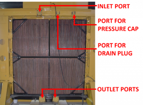
The radiators consist of two principal parts: The heat transfer section and the structural section shown on Figure 1(a). The specifications are shown in Table 2. The heat transfer section is made up of the copper finned-flat tubes. These are installed with rubber seals to the structural section shown on Figure 1(b). These are prone to vibrations caused by the engine, so usually have an intermediate support. The structural section is made up of hard steel plates. There are three tanks (top, bottom and intermediate) where the tubes are installed between each other. There are performance components in the structural section as drain plug, pressure cap, inlet from engine, and outlet to engine shown in Figure 1(c).

A model of a finned-flat tube section is given on Figure 2. All the symbols that are shown are the structural parameters described in Table 3.

1a.png

(a)

1b.png

(b)

1c.png

(c)

Figure 1. Heavy duty truck radiator schematic

2.png

Figure 2. Geometry of finned-flat tube section

Table 3. Structural parameters of finned-flat tubes

2.2 Experimental procedur

In this study the parameters were measured in the field. The study was developed in the southwest area of the department of Arequipa, in Peru. The environmental parameters are shown in Table 4.

Table 4. Environmental parameters

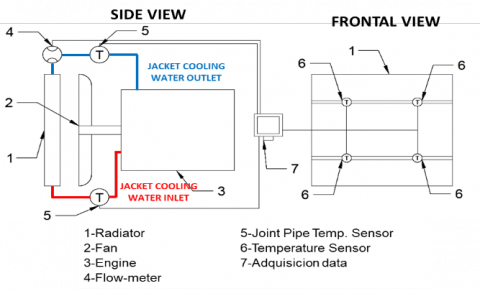
Every heavy-duty equipment usually has a control monitoring system that shows information about the cooling system like temperature and performance of components. The experimental set-up shown in Figure 3 has measurement instruments to evaluate the radiator performance independently of the other system before mentioned. The accuracy for the instruments used to evaluate the radiators are shown in Table 5.

Table 5. Instruments range and accuracy

3.png

Figure 3. Schematic diagram of experimental set-up

The fan is attached to a hydraulic motor. This motor is programmed to increase or reduce rotation speed in function of: Jacket water coolant temperature, Charge air Cooler coolant temperature, Transmission lubrication temperature, Torque converter oil temperature, Brake oil temperature, Brake status, Ground speed, Output status of the hoist system.

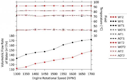
The output parameters measured are shown in Figure 4. The measured points were taken as a function of engine rotation speed. It is considered nine points from each Engine – Radiator group from 1300 RPM to 1700 RPM.

4.jpg

Figure 4. Experimental taken data

In the description WF means Water Flow, WIT means Water Inlet Temperature, WOT means Water Outlet Temperature, AIT means Air Inlet Temperature, and AOT means Air Outlet Temperature. Characteristics ended by 1 are the Engine 1 – Radiator 1 group, and ended by 2 are the Engine 2 – Radiator 2 group. These measured points are not completely accurate due to deviations in engine acceleration. It has been adjusted since the heavy duty trucks tested have an Engine Control Module (ECM) system that can be connected to a computer and digitally obtain engine rotational speed. So that the truck operator can partially simulates a dynamometer.

2.3 Engineering analysis

2.3.1 Finned-flat tube characterization

The geometries of the finned flat tube in the water side are a very common flat tube with rounded ends. On the other hand, on the air side some considerations are needed. Kays and London give some geometrical properties for some finned circular and flat tubes [8]. However, in this situation every tube is considered as an individual heat exchanger.

Air-side heat transfer area per unit length in Eq. (6) is the first step to relate the heat of the process and the overall heat transfer coefficient. It is necessary to parametrize a referential longitudinal section given in Eq. (1) that is a section of the flat tube considering the length of a closed and an opened fin space “s” with fin thickness “t”.

$L_{r e f}=2(s+t)$              (1)

Air-side heat transfer area is calculated by considering all surfaces where air will pass in the longitudinal section: frontal and longitudinal surfaces of fin and the external area of the flat tube. So is needed to solve the frontal area in Eq. (2), longitudinal area in Eq. (3) and external tube area in Eq. (4). It is calculated as follows:

$A_{f}=4[(h+t) t+s t]$            (2)

$A_{l}=2 l(2 s+2 h+t)$            (3)

$A_{t}=\pi D L_{r e f}$               (4)

$A_{T}=2\left(A_{f}+A_{l}\right)+A_{t}$            (5)

$a^{\prime \prime}=\frac{A_{T}}{L_{r e f}}$             (6)

Hydraulic diameter of the heat exchanger in the water side in Eq. (7) is calculated with a simple relation between the wet surface and the flow area inside of the flat tube.

$D_{h, w}=4\left(\frac{d(l-d)+\pi \frac{d^{2}}{4}}{2(l-d)+2 \pi \frac{a}{2}}\right)$                 (7)

In the air side, hydraulic diameter in Eq. (8) will be evaluated in the referential longitudinal section as an average of the two hydraulic diameters in the closed and opened fin space of the longitudinal section.

$D_{h, a}=\frac{4}{2}\left(\frac{s h}{2(s+h)}+\frac{s h}{s+2 h}\right)$                (8)

2.3.2 Heat transfer analysis

The water mass flow is defined in Eq. (9):

$\dot{m}_{w}=\dot{V}_{w} \rho_{w}$              (9)

The heat balance in the air side and the water side is as follows in Eq. (10) and Eq. (11) respectively:

$Q=\dot{m}_{w} c_{w}\left(T_{W O}-T_{W I}\right)$               (10)

$Q=\dot{m}_{a} c_{a}\left(T_{A I}-T_{A O}\right)$           (11)

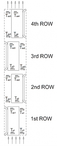
To solve that every tube is considered as an individual heat exchanger, it is needed to separate every row. Figure 5 shows a sectioned projected view in the air side that considers the mass air flow distribution. The purpose is to determine the estimated outlet temperatures of each heat exchanger.

5.png

Figure 5. Schematic of flow balance for each row

Eq. (12) represents the mass air flow passing through the fins and spaces between the finned tubes in a longitudinal section. Eq. (13) is the mass air flow through the fins and Eq. (14) is the mass air flow through the space between finned tubes.

$\dot{m}_{a 1,2}=\frac{\left(\frac{\dot{m}_{a}}{4}\right) 9.75}{19.5\left(\frac{n_{\text {tubes }}}{8}-1\right)+\frac{19.5}{2}}$                (12)

$\dot{m}_{a 1}=\frac{6}{9.75} \dot{m}_{a 1,2}$              (13)

$\dot{m}_{a 2}=\frac{3.75}{9.75} \dot{m}_{a 1,2}$              (14)

Air side heat balance in the first row is developed in Eq. (15), in the second row is developed in Eq. (16), in the third row is developed in Eq. (17), and in the fourth row is developed in Eq. (18).

$\dot{m}_{a 1} h_{T a x 1}+\dot{m}_{a 2} h_{T a 1}=\dot{m}_{a 2} h_{T a x 1}+\dot{m}_{a 1} h_{T a 2}$              (15)

$\dot{m}_{a 1} h_{T a x 2}+\dot{m}_{a 2} h_{T a x 1}=\dot{m}_{a 2} h_{T a x 2}+\dot{m}_{a 1} h_{T a 3}$           (16)

$\dot{m}_{a 1} h_{\text {Tax3 }}+\dot{m}_{a 2} h_{\text {Tax2 } 2}=\dot{m}_{a 2} h_{\text {Tax 3 }}+\dot{m}_{a 1} h_{\text {Ta4 }}$            (17)

$\dot{m}_{a 1} h_{T a x 4}+\dot{m}_{a 2} h_{T a x 3}=\dot{m}_{a 2} h_{T a x 4}+\dot{m}_{a 1} h_{T_{A O}}$               (18)

The mass velocity and Reynolds number on both sides is evaluated in Eq. (19) and (20). The mass velocity is considered per unit on each side. On the water side per tube, and on the air side per fin spacing.

$G=\frac{\dot{m}_{u n i t}}{A_{u n i t}}$               (19)

$\mathrm{Re}=\frac{D_{h} G}{\mu}$                  (20)

On the water side, the Nusselt number will be calculated with the Gnielinski correlation by Eq. (21), which is presented by Bejan [18]. Gnielinski [19] developed this Hausen type correlation to take a large range of liquids with a good accuracy, without considering friction factor.

$N u_{w}=0.012\left(\mathrm{Re}_{w}^{0.87}-280\right) \operatorname{Pr}_{w}^{0.4}$

$1.5 \leq \operatorname{Pr} \leq 500 \ldots .3 \times 10^{3} \leq \operatorname{Re} \leq 10^{6}$              (21)

Convective heat transfer coefficient of water is defined in Eq. (22):

$h_{w}=\frac{N u_{w} k_{w}}{D_{h, w}}$          (22)

LMTD Method is considered as a model to evaluate the air side heat transfer coefficient, considering that will result a different temperature per row. In Eq. (23) “n” means the row number evaluated, and “F” as the crossflow factor.

$\Delta {{T}_{lm}}=F\times \frac{({{T}_{WI}}-{{T}_{axn}})-(\frac{{{T}_{WI}}+{{T}_{WO}}}{2}+{{T}_{an}})}{\ln [\frac{{{T}_{WI}}-{{T}_{axn}}}{\frac{{{T}_{WI}}+{{T}_{WO}}}{2}+{{T}_{an}}}]}$                  (23)

Overall Heat Transfer Coefficient is defined in Eq. (24):

 $U=\frac{Q}{L_{\text {fined }} \times a^{\prime \prime} \times \Delta T_{\text {lm }}}$             (24)

Convective heat transfer coefficient of air has to be calculated with the overall heat transfer coefficient, surface fin effectiveness and relation between water side heat transfer surface and air side heat transfer surface.

Fin effectiveness parameter in Eq. (25) is calculated with air-side convective heat transfer coefficient, heat transfer coefficient of copper and the fin thickness.

Fin efficiency in Eq. (26) is calculated with the fin effectiveness parameter, fin height and fin thickness.

Surface effectiveness of the fins in Eq. (27) is part of the heat transfer coefficient balance, it is calculated with fin efficiency and Fin area/total area relation.

$m_{f}=\sqrt{\frac{2 h_{a}}{k_{\text {copper }} t}}$               (25)

$\eta_{f}=\frac{\tanh \left(m_{f}(h+t)\right)}{m_{f}(h+t)}$              (26)

$\eta_{o}=1-\frac{A_{f}}{A_{T}}\left(1-\eta_{f}\right)$             (27)

So, convective heat transfer coefficient of the air is defined in Eq. (28):

${{h}_{a}}=\frac{1}{{{\eta }_{o}}(\frac{1}{U}-\frac{1}{{{h}_{w}}\frac{{{A}_{w}}}{{{A}_{a}}}})}$                   (28)

2.3.3 Uncertainty analysis

The uncertainties associated with the Heat transfer rate (Eq. (29)), mass air flow (Eq. (30)), Reynolds Number (Eq. (31)), Air side Overall heat transfer coefficient (Eq. (32)), Air side convective heat transfer coefficient (Eq. (34)) were calculated by the following equations [20]. The uncertainties are summarized in Table 6.

Table 6. Uncertainties for the calculated parameters

$\varepsilon_{Q}=\sqrt{\left(\frac{\partial Q}{\partial \dot{m}_{w}} \varepsilon_{m_{w}}\right)^{2}+\left(\frac{\partial Q}{\partial c_{w}} \varepsilon_{c_{w}}\right)^{2}+\left(\frac{\partial Q}{\partial \Delta T_{w}} \varepsilon_{\Delta T_{w}}\right)^{2}}=\sqrt{\left(c_{w} \cdot \Delta T_{w} \cdot \varepsilon_{m_{w}}\right)^{2}+\left(\dot{m}_{w} \cdot \Delta T_{w} \cdot \varepsilon_{c_{w}}\right)^{2}+\left(c_{w} \cdot \dot{m}_{w} \cdot \varepsilon_{\Delta T_{w}}\right)^{2}}$                   (29)

where, Q is the heat transfer rate, m_w is the mass water flow rate, c_w is the water specific heat, ΔT_w is temperature variation between the outlet and inlet temperatures in the water side, and ε_Q, ε_mw, ε_cw and ε_ΔTw are the uncertainties associated with the heat transfer rate, mass flow rate, specific heat and variation between the outlet and inlet temperatures in the water side, respectively.

$\varepsilon_{\dot{m}_{a}}=\frac{\sqrt{\left(\frac{\partial \dot{m}_{a}}{\partial Q} \varepsilon_{Q}\right)^{2}+\left(\frac{\partial \dot{m}_{a}}{\partial c_{a}} \varepsilon_{c_{a}}\right)^{2}+\left(\frac{\partial \dot{m}_{a}}{\partial \Delta T_{a}} \varepsilon_{\Delta T_{a}}\right)^{2}}}{c_{a}^{2} \Delta T_{a}^{2}}=\frac{\sqrt{\left(c_{a} \cdot \Delta T_{a} \cdot \varepsilon_{Q}\right)^{2}+\left(\Delta T_{a} \cdot Q \cdot \varepsilon_{c_{a}}\right)^{2}+\left(c_{a} \cdot Q \cdot \varepsilon_{\Delta T_{a}}\right)^{2}}}{c_{a}^{2} \Delta T_{a}^{2}}$                 (30)

where, m_a is the mass air flow rate, Q is the heat transfer rate, c_a is the air specific heat, ΔT_a is temperature variation between the outlet and inlet temperatures in the air side, and ε_mw, ε_Q, ε_ca and ε_ΔTa are the uncertainties associated with mass air flow rate, heat transfer rate, air specific heat and variation between the outlet and inlet temperatures in the air side, respectively.

$\varepsilon_{\mathrm{Re}}=\frac{\sqrt{\left(\frac{\partial \mathrm{Re}}{\partial D_{h}} \varepsilon_{D_{h}}\right)^{2}+\left(\frac{\partial \mathrm{Re}}{\partial G} \varepsilon_{G}\right)^{2}+\left(\frac{\partial \mathrm{Re}}{\partial \mu} \varepsilon_{\mu}\right)^{2}}}{\mu^{2}}=\frac{\sqrt{\left(\mu \cdot G \cdot \varepsilon_{D_{h}}\right)^{2}+\left(\mu \cdot D_{h} \cdot \varepsilon_{G}\right)^{2}+\left(D_{h} \cdot G \cdot \varepsilon_{\mu}\right)^{2}}}{\mu^{2}}$             (31)

where, Re is the Reynolds Number, D_h is the Hydraulic diameter, G is the mass flow velocity, μ is the dynamic viscosity, and ε_Re, ε_Dh, ε_G, ε_μ are the uncertainties associated with Reynolds Number, Hydraulic diameter, mass flow velocity and dynamic viscosity, respectively.

$\varepsilon_{U_{a}}=\frac{\sqrt{\left(\frac{\partial U_{a}}{\partial Q} \varepsilon_{Q}\right)^{2}+\left(\frac{\partial U_{a}}{\partial A} \varepsilon_{A}\right)^{2}+\left(\frac{\partial U_{a}}{\partial \Delta T_{l m}} \varepsilon_{\Delta T_{l n}}\right)^{2}}}{A^{2} \Delta T_{l m}{ }^{2}}=\frac{\sqrt{\left(\Delta T_{l m} \cdot A \cdot \varepsilon_{Q}\right)^{2}+\left(\Delta T_{l m} \cdot Q \cdot \varepsilon_{A}\right)^{2}+\left(Q \cdot A \cdot \varepsilon_{\Delta T_{l m}}\right)^{2}}}{A^{2} \Delta T_{l m}{ }^{2}}$                (32)

where, U_a is the Overall Heat Transfer coefficient on the air-side, Q is the heat transfer rate, A is the Heat Transfer Surface Area, ΔT_lm is log mean temperature difference, and ε_Ua, ε_Q, ε_A, ε_ΔTlm are the uncertainties associated with the overall heat transfer coefficient on the air side, heat transfer rate, heat transfer surface area and log mean temperature difference, respectively.

$S=\frac{h_{w} A_{w}}{A_{a}}$

$\varepsilon_{S}=\frac{\sqrt{\left(A_{w} \cdot A_{a} \cdot \varepsilon_{h_{w}}\right)^{2}+\left(A_{a} \cdot h_{w} \cdot \varepsilon_{A_{w}}\right)^{2}+\left(h_{w} \cdot A_{w} \cdot \varepsilon_{A_{a}}\right)^{2}}}{A_{a}^{2}}$             (33)

$\varepsilon_{h_{a}}=\frac{\sqrt{\left(\frac{\partial h_{a}}{\partial\left(\frac{1}{U}-\frac{1}{S}\right)}\right)^{2} \times\left(\sqrt{\left(\frac{\varepsilon_{U}}{U^{2}}\right)^{2}+\left(\frac{\varepsilon_{S}}{S^{2}}\right)^{2}}\right)+\left(\frac{\partial h_{a}}{\partial \eta_{o}} \varepsilon_{\eta_{o}}\right)^{2}}}{\left(\eta_{o}\left(\frac{1}{U}-\frac{1}{S}\right)\right)^{2}}=\frac{\sqrt{\left(\eta_{o}\right)^{2} \times\left(\sqrt{\left(\frac{\varepsilon_{U}}{U^{2}}\right)^{2}+\left(\frac{\varepsilon_{S}}{S^{2}}\right)^{2}}\right)+\left(\left(\frac{1}{U}-\frac{1}{S}\right) \cdot \varepsilon_{\eta_{0}}\right)^{2}}}{\left(\eta_{o} \cdot\left(\frac{1}{U}-\frac{1}{S}\right)\right)^{2}}$               (34)

where, h_a is the Air convective heat transfer coefficient, U is the Overall heat transfer coefficient, S is the relation between h_w (Water convective heat transfer coefficient), A_w (Water side surface area) and A_a (Air side surface area) shown in Eq. (33), η_o is the Surface fin effectiveness, and ε_ha, ε_U, ε_S, ε_ηo are the uncertainties associated with the air convective heat transfer coefficient, relation between h_w, A_w and A_a and surface fin effectiveness, respectively.

In this paper, it is shown the air side heat transfer performance of copper finned-flat tubes in flexible core radiators for heavy-duty trucks that has been evaluated in the field. The following are the key findings of this study:

-The thermal design of the two engine-radiator groups evaluated is not uniform. This is because there are variations of the maximum and minimum Reynolds number in both cases. The term “uniform” means a more effective cooling performance with less noise. So that the radiators must be redesigned [7] to achieve a good performance.

-The air convective heat transfer coefficient that was obtained is lower than in conventional compact aluminum radiators [6]. This is because finned-flat tube radiators have a greater heat transfer surface per unit length. And copper as a material of fins increases the fin efficiency.

-The radiator was tested with water as the coolant. Then the results obtained from the Air-side heat transfer coefficient are higher. If water had been used with some other additive or nanofluids [21] the result would be less noise in the variations of this coefficient and thus avoid an irregular behavior.

-The electronic fan drive system has many deviations. Since the hydraulic motor has been programmed to be in constant change due to the other equipment besides the radiator. Therefore, maintaining a stable behavior of the measures taken in the field is very difficult.

It is recommended that for a future study the thermal capacity of these copper finned-flat tubes can be analyzed on a test bench with multiple environmental conditions, to be able to identify if this type of design has better working conditions in different environments. Also, this test bench should be integrated with a system that generates the vibrations of the internal combustion engine and the environment, to be more severe and identify if the structural behavior influences the heat transfer of these radiators.