Hassan El Harfi | Mourad Kaddiri | Mohamed Lamsaadi | Youssef Tizakast*
© 2021 IIETA. This article is published by IIETA and is licensed under the CC BY 4.0 license (http://creativecommons.org/licenses/by/4.0/).
OPEN ACCESS
The present work analyzes both numerically and analytically mixed convection heat transfer in shallow rectangular enclosure files confining ferrofluid, and exposed to temperature conditions of Neuman type with uniform heat flux applied to the short vertical sides, while the top wall is moving with a uniform velocity in the same direction as the applied heat flux. The finite volume method and the SIMPLER algorithm were used to numerically solve the governing equations, while the analytical solution is based on the parallel flow approximation. Simulations are conducted a wide range of controlling parameters, namely, the Reynolds, Hartmann and Richardson numbers and the solid volume fraction of ferroparticles. Effects of mentioned parameters, on the flow structure, temperature fields, and heat transfer rate, were studied and discussed.
ferrofluid, finite volume method, heat transfer, lid-driven enclosure, magnetic field, mixed convection, parallel flow
Ferrofluids are colloidal liquids of nanometric particles of ferromagnetic stably suspended in carrier liquid. By stability we refer to the fact that the suspension remains permanently homogenous, meaning that the particles remain unseparated from the carrier liquid and do not settle at the bottom of the container (do not sediment), nor creates mutual aggregations. To avoid the said aggregations, a stabilizer is used to cover the particles. Each magnetic particle is commonly assimilated to a sphere which is a magnetic dipole. The dipole can be oriented according to the presence of an external magnetic field. In the absence of the magnetic field, the ferrofluids have properties similar to nanofluids. When a field is applied, the behavior of the ferrofluid is changed. Ferrofluid is a liquid that becomes strongly magnetized when a magnetic field is applied. Owing to strong interaction between base fluid and magnetic nanoparticles, the ferrofluid shows surprising thermophysical properties when affected by a magnetic field. Thus, the liquid gains a magnetic behavior from the nanoparticles allowing to the assembly of liquid and nanoparticles to acquire the magnetic behavior.
Given its wide and central technological applications, chemist and physicists spared no effort throughout the last century to produce stable magnetic fluids. Many of those applications are built on the following properties of magnetic fluids: at suitable frequencies, they absorb electromagnetic energy and heat up, go where the strongest magnetic field is, and finally, when subjected to a magnetic field the physical properties may change. Thanks to the mentioned properties, materials and engineering research, technological applications, biology and medical research are all fields that make use of magnetic fluids. The process begins with Chemists who synthesize ferrofluids, while the physicists study and explain the physical properties, then their applicability is investigated and how suitable they are to be applied in practice.
The few studies (rheological, thermal, magnetic ...) carried out on ferrofluids, present them a priori as fluids eligible for the intensification of heat exchanges. However, the discrepancies between these studies do not allow a conclusion to be drawn on the real potential of these fluids, in particular for application in cooling systems.
The thermal characterization of ferrofluids under magnetic field for cooling applications necessarily involves the determination of the coefficient of convection denoted h. We have therefore investigated the literature on this aspect. Most studies show local improvements in the convection coefficient, indicating an intensification of heat exchange. These improvements are essentially achieved with laminar flows. Moreover, we also notice that the nature of the magnetic field applied affects the coefficient h. Several field configurations are identified. However, a few studies have been carried out to explain the origin of the improvement of h, compared with the case without field. Even so, this point remains at the hypothetical stage.
As in the case of a nanofluid, the thermal conductivity of a ferrofluid depends on several parameters, namely: ferroparticles volume fraction, their size, the nature of the base fluid, and the intensity of the magnetic field. Recent studies have shown a significant improvement in the thermal conductivity coefficient of ferrofluids when subjected to magnetic field. The results of the work of Philip et al. [1] represent the thermal conductivity ratio of the ferrofluid and that of the base fluid. By increasing the intensity of the magnetic field, the thermal conductivity increases. The same reasoning applies to the volume fraction. The improvement thus obtained reaches 130% with respect to the base fluid. Gavili et al. [2] measured the conductivity of a ferrofluid with a water-based carrier fluid containing 5% Fe3O4 ferroparticles. Their results show a 200% increase in the thermal conductivity coefficient. Studies on the convective coefficient of exchange of ferrofluids are promising. Lajvardi et al. [3] experimentally studied the convective coefficient of exchange for a ferrofluid at different concentrations. They conclude that, due to the increase in concentration and the magnetic field, the ferrofluid’s thermal capacity along with its thermal conductivity are increased and as a result, the heat exchanges are better (improvements up to 30% compared with the ferrofluid without field).
Most studies inspecting heat transfer of ferrofluids have considered the phenomena of natural convection, while mainly focusing on the numerical work [4]. Rudraiah et al [5] numerically examined natural convection with applied magnetic field parallel to gravity of electrically conducting fluid. The study inspects how the strength of the magnetic field affects the flow structure inside a cavity. Jafari et al. [6] numerically studied heat transfer of a kerosene based ferrofluid in two cylinders with different geometries. They found that the heat transfer depends on both the magnetic field strength and direction. On the other hand, increasing the magnetic particles’ diameter decreases heat transfer. Khanafer et al. [7] investigated heat transfer enhancement numerically in a two-dimensional cavity. The results showed that increasing the nanoparticles volume fraction increases the heat transfer rate, and that their presence in the fluid change the fluid flow structure. Yamaguchi et al. [8] studied natural convection of a magnetic fluid inside three-dimensional cavity both experimentally and numerically. The results showed that applying a magnetic field enhances heat transfer, while increasing the field strength increases heat transfer further. Meherz and El Cafsi [9] used the finite volume method to numerically examine natural heat exchange of ferrofluids in the presence of a magnetic field. They showed that both inserting ferromagnetic nanoparticles and applying a magnetic field leads to 86% increases in heat exchange, while adding ferro-particles alone leads only to 20% increase. Sheikholeslami and Vajravelu [10] studied the influence of a variable magnetic field on flow and heat transfer of a nanofluid. They found that increasing Lorentz force increases heat transfer rate while buoyancy force produces the opposite effect. Szabo and Früh [11] investigated the transition from natural convection to thermomagnetic convection numerical of a magnetic fluid subjected to a non-uniform magnetic field. Yamaguchi et al. [12] analyzed flow and heat transfer characteristics of magnetic fluid natural convection inside a two-dimensional cavity. They found that the vertical magnetic field has a destabilizing effect on the flow transition as the critical Rayleigh number decreased when the field is applied. Cheng and Li [13] studied the heat transfer characteristics of diester-based ferrofluid natural convection in a horizontal channel under a permanent magnetic fluid. On the other hand, Bian et al. [14] considered an inclined rectangular porous enclosure saturated with an electrically conducting fluid to examine the outcome on buoyancy-driven convection when subjected to a transverse magnetic field. There are many other studies that explores the results of applied magnetic field on natural convection heat transfer for cavities filled with ferrofluids, that we cite here to refer to for more details [15-20].
Mixed convection on the other hand, attracted less interest compared to natural one, even that it is present in a widely range of applications such as heat transfer in solar ponds, cooling technics, glass production, food processing, and many others. Mixed convection is due to both buoyancy force that results from thermal gradient and shear force caused by the moving walls. Studies [21-23] considered different combinations of cavities and imposed temperature gradients. Abu-Nada and Chamkha [24] conducted a numerical study of the characteristics of heat transfer in an inclined square encloser with moving top wall, they found that those characteristics improved due to the presence of nanoparticles. Mahmoudi [25] investigated heat transfer in a rectangular enclosure occupied with nanofluid while the bottom wall is moving, the results show that the Nusselt number enhances when increasing volume fraction of the nanoparticles. Gibanov et al. [26] numerically studied ferrofluid mixed convection in a lid-driven square cavity under the effect of a uniform inclined magnetic field. The conclusions showed that the magnetic field inclination can be used to control heat transfer enhancement. On the other hand, increasing Hartman number decreased the average Nusselt number. Hekmat et al. [27] investigated magnetic field gradient on thermomagnetic mixed convection of a ferrofluid in a three- dimensional annular space between two cylinders. While a negative magnetic field gradient increased friction coefficient and the Nusselt number on the inner wall, a magnetic field with a positive gradient leads to the opposite effect as both characteristics reduce. Job and Gunakala [28] analyzed mixed convection flow of a water-based ferrofluid in a wavy channel with two porous blocks mounted on the heated sections of the walls under the effect of an alternating magnetic field. They found that when the porous block thickness increases in a small values range, The average Nusselt number reduces, while the opposite is true when the thickness increases through large values. Mehmoud [29] conducted a numerical study thermomagnetic convection within lid-driven trapezoidal cavities occupied with a kerosene‑cobalt ferrofluid. The results showed that the fluid flow strongly depends on ferro particles concentration, Grashof, Darcy, and Hartman numbers. Sheikholeslami and Chamkha [30] studied the influence of a variable magnetic field on heat transfer in a double lid-driven cavity with a wavy hot wall and filled with a ferro-nanofluid. They found that increasing the magnetic number, Reynolds number, and the volume fraction of particles increases Nusselt number, while increasing Hartmann number leads to an inverse trend.
The review of the literature shows clearly that a minor share of investigations considers the effect of magnetic field on mixed convection. Furthermore, most of the existing studies treated the case of imposed temperatures at the active walls. Hence, the problem of mixed convection in a rectangular cavity with thermal boundary conditions of Neumann Type (i.e., imposed heat flux) has not been studied yet. To fill in the gap, the present study considers a two-dimensional shallow rectangular cavity occupied with Co-water ferrofluids, the short vertical walls are subjected to uniform heat fluxes whereas the horizontal ones are adiabatic with the top wall is sliding in the same direction of the applied heat flux, the main objective is to inspect the effect of the magnetic field on heat transfer characteristics. As we mentioned before, the majority of studies presented a numerical solution of the problem, while in our case, two solutions were adopted, a numerical solution of the full governing equations using finite volume method plus an analytical one build upon the parallel flow approximation. The results are given in terms of stream function, Nusselt number, streamlines, isotherms, and temperature profiles for a wide range of controlling dimensionless parameters, namely: Reynolds number, $R e$, Hartmann number, $H a$, Richardson number, Ri, and the solid volume fraction of nanoparticles, $\Phi$. The paper first introduces the governing equations of the problem, then details the numeric method before elaborating the analytical approach. Finally, both methods are compared against each other to verify their agreement and the effect of governing parameters on flow characteristics and heat transfer is discussed. This study seeks to strengthen the literature on ferrofluids mixed convection.
The considered configuration is outlined in Figure 1. A shallow rectangular cavity with length L’ and height H’, occupied with Co-water ferrofluids. The long horizontal walls are adiabatic and the top one is sliding with a constant velocity, whereas the vertical ones are subjected to a uniform density of heat flux, q’. The four walls are rigid and impermeable.
The frequently used assumptions in such problems are expressed as follows:
Using the mentioned assumptions above, the governing equations expressing the conservation of mass (1), momentum (2)-(3) and energy (4), are given in terms of velocity components $\left(u^{\prime}, v^{\prime}\right)$, pressure $\left(p^{\prime}\right)$ and temperature $\left(T^{\prime}\right)$:
$\frac{\partial u^{\prime}}{\partial x^{\prime}}+\frac{\partial v^{\prime}}{\partial y^{\prime}}=0$ (1)
Figure 1. Sketch of the cavity and co-ordinates system
$\frac{\partial u^{\prime}}{\partial t^{\prime}}+u^{\prime} \frac{\partial u^{\prime}}{\partial x^{\prime}}+v^{\prime} \frac{\partial u^{\prime}}{\partial y^{\prime}}=-\frac{1}{\rho_{f f}} \frac{\partial p^{\prime}}{\partial x^{\prime}}+\frac{\mu_{f f}}{\rho_{f f}}\left(\frac{\partial^{2} u^{\prime}}{\partial x^{\prime}}+\frac{\partial^{2} u \prime}{\partial y^{\prime 2}}\right)+$$\frac{\sigma_{f f} B^{2}}{\rho_{f f}}\left(v \sin \theta \cos \theta-u \sin ^{2} \theta\right)$ (2)
$\frac{\partial v^{\prime}}{\partial t^{\prime}}+u^{\prime} \frac{\partial v^{\prime}}{\partial x^{\prime}}+v^{\prime} \frac{\partial v^{\prime}}{\partial y^{\prime}}=-\frac{1}{\rho_{f f}} \frac{\partial p^{\prime}}{\partial y^{\prime}}+\frac{\mu_{f f}}{\rho_{f f}}\left(\frac{\partial^{2} v_{1}}{\partial x_{\prime}^{2}}+\frac{\partial^{2} v \prime}{\partial y^{\prime}}\right)+$$\frac{1}{\rho_{f f}}(\rho \beta)_{f f} g\left(T^{\prime}-T_{0}^{\prime}\right)+\frac{\sigma_{f f}^{B^{2}}}{\rho_{f f}}(u \sin \theta \cos \theta-$$\left.v \cos ^{2} \theta\right)$ (3)
$\frac{\partial T^{\prime}}{\partial t^{\prime}}+\frac{\partial\left(u^{\prime} T \prime\right)}{\partial x^{\prime}}+\frac{\partial(v \prime T \prime)}{\partial y \prime}=\alpha_{f f} \nabla^{2} T^{\prime}$ (4)
The associated boundary conditions are:
$u^{\prime}=v^{\prime}=0$ and $\frac{\partial T^{\prime}}{\partial x^{\prime}}+\frac{q^{\prime}}{k_{f f}}=0$ for $x^{\prime}=0$ and $x^{\prime}=L^{\prime}$ (5)
$u^{\prime}=v^{\prime}+U_{0}^{\prime}=0$ and $\frac{\partial T^{\prime}}{\partial y^{\prime}}=0$ for $y^{\prime}=0$ (6)
$u^{\prime}-U_{0}^{\prime}=v^{\prime}=0$ and $\frac{\partial T^{\prime}}{\partial y^{\prime}}=0$ for $y^{\prime}=H^{\prime}$ (7)
The next formulations are used to define the ferrofluid effective physical properties emerged in the above governing equations.
The constant density of ferrofluid can be descried as follows,
$\rho_{f f}=(1-\Phi) \rho_{f}+\Phi \rho_{s}$ (8)
Next, the ferrofluid dynamic viscosity μff and can be defined as,
$\mu_{f f}=\frac{\mu_{f}}{(1-\Phi)^{2.5}}$ (9)
The thermal expansion coefficient (ρβ)ff,
$(\rho \beta)_{f f}=(1-\Phi)(\rho \beta)_{f}+\Phi(\rho \beta)_{s}$ (10)
The heat capacitance of ferrofluid ,
$(\rho C p)_{f f}=(1-\Phi)(\rho C p)_{f}+\Phi(\rho C p)_{s}$ (11)
As for the Effective thermal conductivity, owing to Maxwell-Garnett, which is a restriction of the Hamilton-Crosser model to spherical ferroparticles according to Yu et al. [31], it can be defined as,
$\frac{k_{f f}}{k_{f}}=\frac{k_{S}+2 k_{f}-2 \Phi\left(k_{f}-k_{S}\right)}{k_{S}+2 k_{f}+\Phi\left(k_{f}-k_{S}\right)}$ (12)
The ferrofluid thermal diffusivity is rather different from the base fluid and can be written as follows,
$\alpha_{f f}=\frac{k_{f f}}{(\rho C p)_{f f}}$ (13)
Finally, Maxwell [32] described the ferrofluid effective electrical conductivity as shown below:
$\bar{\sigma}=\frac{\sigma_{f f}}{\sigma_{f}}=1+\frac{3\left(\frac{\sigma_{S}}{\sigma_{f}}-1\right) \varphi}{\left(\frac{\sigma_{S}}{\sigma_{f}}+2\right)+\left(\frac{\sigma_{S}}{\sigma_{f}}-1\right) \varphi}$ (14)
On the other hand, Table 1 shows the thermophysical properties of both base fluid (Water) and the ferromagnetic particle (Cobalt) adopted for the present study.
The following dimensionless equations and the associated boundary conditions are obtained using the appropriate characteristic scales $H^{\prime}, \rho_{f} U_{0}^{\prime 2}, H^{\prime} / U_{0}^{\prime}, U_{0}^{\prime}$, and $q^{\prime} H^{\prime} / k_{f}$, for length, pressure, time, velocity, and temperature, respectively.
$\frac{\partial u}{\partial x}+\frac{\partial v}{\partial y}=0$ (15)
$\frac{\partial u}{\partial t}+u \frac{\partial u}{\partial x}+v \frac{\partial u}{\partial y}=-\frac{1}{\bar{\rho}} \frac{\partial p}{\partial x}+\frac{\bar{v}}{R e}\left(\frac{\partial^{2} u}{\partial x^{2}}+\frac{\partial^{2} u}{\partial y^{2}}\right)+$$\frac{\bar{\sigma}}{\bar{\rho}} \frac{H a^{2}}{R e}\left(v \sin \theta \cos \theta-u \sin ^{2} \theta\right)$ (16)
$\frac{\partial v}{\partial t}+u \frac{\partial v}{\partial x}+v \frac{\partial v}{\partial y}=-\frac{1}{\bar{\rho}} \frac{\partial p}{\partial y}+\frac{\bar{v}}{R e}\left(\frac{\partial^{2} v}{\partial x^{2}}+\frac{\partial^{2} v}{\partial y^{2}}\right)+$$\frac{\bar{\beta}}{\bar{\rho}} R i T+\frac{\bar{\sigma}}{\bar{\rho}} \frac{H a^{2}}{\operatorname{Re}}\left(u \sin \theta \cos \theta-v \cos ^{2} \theta\right)$ (17)
$\frac{\partial T}{\partial t}+u \frac{\partial T}{\partial x}+v \frac{\partial T}{\partial y}=\frac{\bar{\alpha}}{P e}\left(\frac{\partial^{2} T}{\partial x^{2}}+\frac{\partial^{2} T}{\partial y^{2}}\right)$ (18)
$u=v=\frac{\partial T}{\partial x}+\frac{1}{\bar{k}}=0$ for $x=0$ and $A$ (19)
$u=v+1=\frac{\partial T}{\partial y}=0$ for $y=0$ (20)
$u-1=v=\frac{\partial T}{\partial y}=0$ for $y=1$ (21)
where:
$\bar{k}=k_{f f} / k_{f} ; \bar{\alpha}=\alpha_{f f} / \alpha_{f} ; \bar{v}=v_{f f} / v_{f}$,
$\bar{\beta}=(\rho \beta)_{f f} /(\rho \beta)_{f} ; \bar{\sigma}=\sigma_{f f} / \sigma_{f}$ and $\bar{\rho}=\rho_{f f} / \rho_{f}$.
They are dependent parameters on Φ, conforming to models specified above.
The previous equations illustrate the governing parameters of flow and heat transfer, namely: the solid volume fraction , the aspect ratio of the cavity, A, plus the Peclet, , Reynolds, , Hartmann and Richardson, , numbers, which can be expressed for the base fluid as follows,
$A=\frac{L^{\prime}}{H^{\prime}}, P e=\frac{U_{0}^{\prime} H^{\prime}}{\alpha_{f}}, \operatorname{Re}=\frac{U_{0}^{\prime} H^{\prime}}{v_{f}}, H a=B H^{\prime} \sqrt{\sigma_{f} / \mu_{f}}$
and $R i=\frac{g \beta_{f} q^{\prime} H^{\prime 2}}{k_{f} U_{0}^{\prime 2}}$ (22)
Note that:
$P e=\operatorname{PrRe}$ and $R i=\frac{G r}{R e^{2}}=\frac{R a}{P e R e}$ (23)
where:
$G r=\frac{g \beta_{f}^{\prime} q^{\prime} H^{\prime 4}}{v_{f}^{2} k_{f}}, P r=\frac{v_{f}}{\alpha_{f}}$ and $R a=\operatorname{Pr} G r$ (24)
Local Nusselt number quantifying the local heat transfer inside an enclosure filled with a ferrofluid is defined as follows:
$\operatorname{Nu}(\mathrm{y})=\frac{\mathrm{hL}^{\prime}}{\mathrm{k}_{\mathrm{f}}}=\frac{\mathrm{q}^{\prime}}{\Delta \mathrm{T}^{\prime}} \frac{\mathrm{L}^{\prime}}{\mathrm{k}_{\mathrm{f}}}=\frac{\mathrm{L}^{\prime}}{\mathrm{H}^{\prime}} \frac{\Delta \mathrm{T}^{*}}{\Delta \mathrm{T}^{\prime}}=\frac{\mathrm{A}}{\mathrm{T}(0)-\mathrm{T}(\mathrm{A})}$ (25)
$h$ refers to the heat exchange coefficient, $\Delta T^{*}=q^{\prime} H^{\prime} / k_{f}$ a characteristic temperature and $\Delta T=T(0, y)-T(A, y)$ is dimensionless temperature difference between the two vertical walls of equations $x=0$ and $x=A$, respectively. For the definition in question, the thermal conductivity of the base fluid, $k_{f}$, is used, which makes sense according to Corcione [33], who showed that for Nusselt number to define the thermal performance inside the cavity, with immediacy, it needs to vary in the same way as h and vice versa. Still, owing to the edge effects problem that emerge near the vertical walls, Eq. (25) faces problems of inaccuracy due to uncertainty of the measured temperature along the said walls.
To solve the problem, Nu is measured using the following expression: $N u(x, y)=\frac{A-2 x}{T(x, y)-T(A-x, y)}$, this expression seems logical because it gives the equation (25) for $x=0$ and gives the one suggested by Lamsaadi et al. [34].
$N u(y)=\lim _{\delta x \rightarrow 0} \frac{\delta x}{\delta T}=\lim _{\delta x \rightarrow 0} \frac{1}{(\delta T / \delta x)}=-\frac{1}{(\partial T / \partial x)_{x=A / 2}}$ when $x \rightarrow \frac{A}{2}$.
The average Nusselt number has the following expression:
$\bar{N} u=\frac{2}{A} \int_{0}^{1} \int_{0}^{\frac{A}{2}} N u(x, y) d x d y=$$\frac{2}{A} \int_{0}^{1} \int_{0}^{A / 2} \frac{A-2 x}{T(x, y)-T(A-x, y)} d x d y$ (26)
The velocity components and are used to define the stream function, which is used to display the flow field structure using streamlines. The stream function is given in terms of velocity components by the following formulas:
$\mathrm{u}=\frac{\partial \Psi}{\partial \mathrm{y}}$ and $\mathrm{v}=-\frac{\partial \Psi}{\partial \mathrm{x}}($ with $\psi=0$ on all boundaries) (27)
Table 1. Thermophysical properties of water and cobalt
|
|
$\boldsymbol{C}_{\boldsymbol{p}}(\boldsymbol{J} /(\boldsymbol{k g} \cdot \boldsymbol{K}))$ |
$\rho\left(k g / m^{3}\right)$ |
$\boldsymbol{k}(\boldsymbol{W} /(\boldsymbol{m} \cdot \boldsymbol{K}))$ |
$\beta\left(K^{-1}\right)$ |
|
H2O |
4185.5 |
1000 |
0.6071 |
5 10-5 |
|
Co |
420 |
8900 |
100 |
1.3 10-5 |
The well-known finite volume method and SIMPLER algorithm in a uniform grid system (Patankar [35]) is adopted to numerically solve the closed system of Eqns. (15)-(18) associated with boundary conditions (19)-(21). The temporal terms emerging from Eqns. (16)-(18) are discretized with a second order back-wards finite difference scheme. To solve the obtained nonlinear discretized equations, a combination of a line-by-line tridiagonal matrix algorithm with relaxation and an iterative process is implemented. The condition $\sum_{i, j}\left|f_{i, j}^{k+1}-f_{i, j}^{k}\right|<10^{-5} \sum_{i, j}\left|f_{i, j}^{k+1}\right|$, where $f_{i, j}^{k}$ denotes the value of $u, v, p$ or $T$ at the kth iteration level and grid point $(i, j)$ in the two-dimensional plan $(x, y)$. Numerical tests were conducted to pick the mesh size with the optimal arrangement between running time and accuracy. The mesh size is refined until a reasonable agreement is found between the numerical results and the analytical ones established based on the parallel flow approach as shown in the next section. A uniform grid of $160 \times 40$ with an aspect ratio $A=16$, is found to be sufficient to accurately model the flow structure and temperature fields inside the enclosure. Given the values of controlling parameters, the time step, $\delta t$, is chosen from the range $10^{-7} \leq$$\delta t \leq 10^{-4}$.
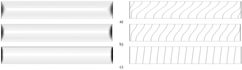
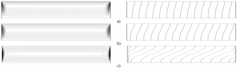
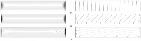
Upon examining Figures 2-4, illustrating streamlines (left) and isotherms (right) for A=16 and several values of $R e, R i, H a$ and $\Phi$, it is observed that for most part of the enclosure, the flow structure shows a parallel aspect while the temperature fields reveal a linear stratification in the vertical direction. Based on those observations, the following simplifications are made
$v(x, y)=0, u(x, y)=u(y), \psi(x, y)=\psi(y)$ and $T(x, y)=C(x-A / 2)+\theta(y)$ (28)
With C is the unknown constant temperature gradient in the x-direction, as a result, the next non-dimensional governing equations are obtained:
$\frac{d^{3} u}{d y^{3}}-(H a \sin \alpha)^{2} \frac{d u}{d y}=\bar{\alpha} \Omega \operatorname{Re} R i \frac{\partial T}{\partial x}$$=\bar{\alpha} \Omega R e R i C$ (29)
$\frac{\bar{\alpha}}{P e} \frac{d^{2} \theta}{d y^{2}}=C u$ (30)
With:
$u+1=\frac{d \theta}{d y}=0$ for $y=0$ and $u-1=\frac{d \theta}{d y}=0$ for $y=1$ (31)
$\int_{0}^{1} u(y) d y=0$ (32)
$\int_{0}^{1} \theta(y) d y=0$ (33)
They are the associated boundary conditions, the return flow and the mean temperature conditions, respectively.
Figure 2. Streamlines (left) and isotherms (right) for $A=16, \operatorname{Re}=1, R i=10^{3}, \Phi=0$ and various values of $H a((a): H a=1,(b): H a=10$ and $(c): H a=50)$
Figure 3. Streamlines (left) and isotherms (right) for $A=16, H a=5, \operatorname{Re}=1, \Phi=0$ and various values of $R i\left((a): R i=10,(b): R i=10^{2}\right.$ and $\left.(c): R i=10^{4}\right)$
Figure 4. Streamlines (left) and isotherms (right) for $A=16, H a=5, R i=10^{3}, \Phi=0$ and various values of $\operatorname{Re}((a): R e=0.1,(b): \operatorname{Re}=1$ and $(c): R e=10)$
Exploiting such an approach, Eqns. (29) and (30), satisfying Eqns. (31), (32) and (33), where $\Omega=\frac{\bar{\beta}}{\bar{\rho} \bar{\alpha} \bar{\nu}}$, are generalized as follows:
$u(y)=C\left(B e^{\omega y}+D e^{-\omega y}-\frac{R i R e}{\omega^{2}} y+E\right)+$$F e^{\omega y}+G e^{-\omega y}+K$ (34)
$\theta(y)=\operatorname{RePrC}^{2}$$\left(\frac{B}{\omega^{2}} e^{\omega y}+\frac{D}{\omega^{2}} e^{-\omega y}-\frac{R i R e}{6 \omega^{2}} y^{3}+\frac{E}{2} y^{2}-X_{1} y+Z_{1}\right)+$$\operatorname{RePrC}\left(\frac{F}{\omega^{2}} e^{\omega y}+\frac{G}{\omega^{2}} e^{-\omega y}+\frac{K}{2} y^{2}-X_{2} y+Z_{2}\right)$ (35)
with:
$B=\frac{R}{K_{1} M_{2}-M_{1} K_{2}}\left(M_{2}-\frac{K_{2}}{2}\right)$; $D=\frac{R}{K_{1} M_{2}-M_{1} K_{2}}\left(\frac{K_{1}}{2}-M_{1}\right)$; $E=-(B+D)$; $F=\frac{2 M_{2}+K_{2}}{K_{1} M_{2}-M_{1} K_{2}}$; $G=\frac{2 M_{1}+K_{1}}{K_{1} M_{2}-M_{1} K_{2}}$;
$K=-(1+F+G)$; $\omega=H a$; $R=\frac{R i R e}{\omega^{2}}$; $X_{1}=\frac{B-D}{\omega}$; $X_{2}=\frac{F-G}{\omega}$;
$Z_{1}=\frac{B-D}{2 \omega}-\frac{B}{\omega^{3}}\left(e^{\omega}-1\right)+\frac{D}{\omega^{3}}\left(e^{-\omega}-1\right)+\frac{R}{24}-\frac{E}{6}$;
$Z_{2}=\frac{F-G}{2 \omega}-\frac{F}{\omega^{3}}\left(e^{\omega}-1\right)+\frac{G}{\omega^{3}}\left(e^{-\omega}-1\right)-\frac{E}{6}$;
$K_{1}=e^{\omega}-1 ; K_{2}=e^{-\omega}-1 ; M_{1}=\frac{e^{\omega}-1-\omega}{\omega}$;
$M_{1}=\frac{e^{\omega}-1-\omega}{\omega}$; (36)
Through integration of equation (27), the stream function, $\psi(y)$ expression is obtained:
$\psi(\mathrm{y})=\mathrm{C}\left(\frac{\mathrm{B}}{\omega}\left(\mathrm{e}^{\omega \mathrm{y}}-1\right)-\frac{\mathrm{D}}{\omega}\left(\mathrm{e}^{-\omega \mathrm{y}}-1\right)-\right.$$\left.\frac{\mathrm{RiRe}}{2 \omega^{2}} \mathrm{y}^{2}+\mathrm{Ey}\right)+\frac{\mathrm{F}}{\omega}\left(\mathrm{e}^{\omega \mathrm{y}}-1\right)-\frac{\mathrm{G}}{\omega}\left(\mathrm{e}^{-\omega \mathrm{y}}-1\right)+\mathrm{Ky}$ (37)
which presents the maximum value of $|\psi(y)|$ in the center vertical region of the cavity $(x=A / 2)$.
As for the energy balance in x-direction, as reported by Bejan [36]:
$\int_{0}^{1}-\frac{\partial \mathrm{T}}{\partial \mathrm{x}} \mathrm{dy}+\operatorname{RePr} \int_{0}^{1} \mathrm{uTdy}=\int_{0}^{1}-\left(\frac{\partial \mathrm{T}}{\partial \mathrm{x}}\right)_{\mathrm{x}=0 \text { or } \mathrm{A}} \mathrm{dy}$ (38)
Particularly, in the parallel flow region and while condition (19) is applied, (39) becomes:
$-C+R e P r \int_{0}^{1} u T d y=1$ (39)
to which replacing $u(y)$ and $\theta(y)$ with their respective expressions, leads to the following transcendental equation:
$(\operatorname{RePr})^{2} \beta_{1} C^{3}+(\operatorname{RePr})^{2} \beta_{2} C^{2}+\left((\operatorname{RePr})^{2} \beta_{3}-1\right)$$C-1=0$ (40)
where, the expression of $\beta_{1}, \beta_{2}$, and $\beta_{3}$ are as follows:
$\beta_{1}=\left(\frac{1}{120 \omega^{4}}\right)\left(\begin{array}{l}60 \mathrm{~B}^{2} \mathrm{e}^{2 \omega} \omega-60 \omega(\mathrm{B}-\mathrm{D})(\mathrm{B}+\mathrm{D}+2 \mathrm{E})-240 \mathrm{R}(\mathrm{B}+\mathrm{D}) \\ +240 \mathrm{BD} \omega^{2}+\mathrm{R} \omega^{4}(4 \mathrm{R}-5 \mathrm{E}) \\ -20 \mathrm{Be}^{\omega}(\mathrm{R}(\omega((\omega-3) \omega+12)-12)-6 \mathrm{E} \omega)-60 \mathrm{D}^{2} \mathrm{e}^{-2 \omega} \omega \\ +20 \mathrm{De}^{-\omega}(\mathrm{R}(\omega(\omega(\omega+3)+12)+12)-6 \mathrm{E} \omega)\end{array}\right)+$
$\left(\frac{1}{24 \omega^{3}}\right)\left(\begin{array}{l}12 \mathrm{~B}\left(\mathrm{E}\left(\mathrm{e}^{\omega}((\omega-2) \omega+2)-2\right)-2 \mathrm{X}_{1}\left(\mathrm{e}^{\omega}(\omega-1)+1\right) \omega\right) \\ +\omega^{3}\left(4 \mathrm{E}^{2}-3 \mathrm{E}\left(4 \mathrm{X}_{1}+\mathrm{R}\right)+8 \mathrm{X}_{1} \mathrm{R}\right) \\ +12 \mathrm{De}^{-\omega}\left(\mathrm{E}\left(-\omega(\omega+2)+2 \mathrm{e}^{\omega}-2\right)+2 \mathrm{X}_{1} \omega\left(\omega-\mathrm{e}^{\omega}+1\right)\right)\end{array}\right)$$+E Z_{1}-\frac{Z_{1}\left(-2 B\left(e^{\omega}-1\right)+2 D e^{-\omega}-2 D+R \omega\right)}{2 \omega}$
$\beta_{2}=\left(\frac{1}{24 \omega^{4}}\right)$$\left(\begin{array}{l}-12 F(\omega(B-2 D \omega+2 E)+2 R)+12 G(\omega(2(B \omega+E)+D)-2 R) \\ +K \omega\left(-24 B+24 D+\omega^{3}(4 E-3 R)\right)-12 e^{\omega}\left(2 F(R(\omega-1)-E \omega)-B K \omega\left(\omega^{2}-2 \omega+2\right)\right) \\ +12 B F e^{2 \omega} \omega+12 e^{-\omega}\left(2 G(-E \omega+R \omega+R)-D K \omega\left(\omega^{2}+2 \omega+2\right)\right)-12 D G e^{-2 \omega} \omega\end{array}\right)-$
$\frac{\mathrm{B}\left(\mathrm{X}_{2}+\mathrm{Z}_{2} \omega\right)}{\omega^{2}}+\frac{\mathrm{Be}^{\omega}\left(-\mathrm{X}_{2} \omega+\mathrm{X}_{2}+\mathrm{Z}_{2} \omega\right)}{\omega^{2}}+\frac{\mathrm{De}^{-\omega}\left(\mathrm{X}_{2} \omega+\mathrm{X}_{2}-\mathrm{Z}_{2} \omega\right)}{\omega^{2}}+\frac{\mathrm{D}\left(\mathrm{Z}_{2} \omega-\mathrm{X}_{2}\right)}{\omega^{2}}+\frac{1}{6}\left(-3 \mathrm{EX}_{2}+6 \mathrm{EZ}_{2}+2 \mathrm{X}_{2} \mathrm{R}-3 \mathrm{Z}_{2} \mathrm{R}\right)+$
$\left(\frac{1}{24 \omega^{4}}\right)$$\left(\begin{array}{l}-12 \omega(B(F+2 K)-D(G+2 K))-24 \omega^{2}(B G+D F)+24 R(F+G)+K R \omega^{4} \\ -4 e^{\omega}(F R(\omega((\omega-3) \omega+6)-6)-6 B K \omega)+12 B F e^{2 \omega} \omega \\ +4 \mathrm{e}^{-\omega}(G R(\omega(\omega(\omega+3)+6)+6)-6 D K \omega)-12 D G e^{-2 \omega} \omega\end{array}\right)+$
$\left(\frac{1}{6 \omega^{3}}\right)$$\left(\begin{array}{l}E\left(-6 F+6 G+K \omega^{3}\right)-3 X_{1} \omega\left(2(F+G)+K \omega^{2}\right)+6 \omega^{2} Z_{1}(-F+G+K \omega) \\ +3 F e^{\omega}\left(E((\omega-2) \omega+2)+2 \omega\left(-X_{1} \omega+X_{1}+Z_{1} \omega\right)\right) \\ -3 G e^{-\omega}\left(E(\omega(\omega+2)+2)-2 \omega\left(X_{1} \omega+X_{1}-Z_{1} \omega\right)\right)\end{array}\right)$
$\beta_{3}=\left(\frac{1}{6 \omega^{3}}\right)$$\left(\begin{array}{l}3 F^{2} e^{2 \omega}-3(F-G)(F+G+4 K)+6 \omega\left(2 F G-X_{2}(F+G)\right)+6 Z_{2} \omega^{2}(G-F) \\ +K \omega^{3}\left(K-3 X_{2}+6 Z_{2}\right)+3 F e^{\omega}\left(K((\omega-2) \omega+4)+2 \omega\left(-X_{2} \omega+X_{2}+Z_{2} \omega\right)\right) \\ -3 G^{2} e^{-2 \omega}-3 G e^{-\omega}\left(K(\omega(\omega+2)+4)-2 \omega\left(X_{2} \omega+X_{2}-Z_{2} \omega\right)\right)\end{array}\right)$ (41)
Lastly, taking into consideration (25) and (26), the Nusselt number is found to be constant and can be written as:
$N u=\overline{N u}=-\frac{1}{c}$ (42)
As for the stream function in the center of the cavity:
$\psi_{c}=\operatorname{Sup}\left(\psi_{\max },\left|\psi_{\min }\right|\right)$ (43)
with $\psi_{\max }$ and $\left|\psi_{\min }\right|$ are the extremums of stream function, $\psi(y)$, at the center vertical region of the cavity $(x=A / 2)$. They present the intensities of forced and natural convection regimes, respectively.
Mixed convection in a two-dimensional shallow rectangular enclosure filled with a Cobalt-water ferrofluid is studied. Temperature boundary conditions of Neuman type (uniform heat flux) are applied to the short vertical sides, while the horizontal ones are insulated with the top one is moving from left to right in the direction of the imposed flow. The study is conducted with $A=16$ and a wide range of the explored parameters, namely: Re $(0.1 \leq \operatorname{Re} \leq 10)$, Ri $(1 \leq R i \leq$ $\left.510^{4}\right), H a(1 \leq H a \leq 80), \Phi(0 \leq \Phi \leq 0.2)$, and $\operatorname{Pr}=7$.
Accordingly, four parameters govern the mixed convection flow inside the cavity: $R e, R i, H a$ and $\Phi$. In what follows, the effects of said parameters on flow structure, temperature field and heat transfer will be illustrated and discussed.
5.1 Validation of the approximate analytical solution
Numerical computations were conducted to find the smallest value of aspect ratio A, that results in flow characteristics to become invariant to the aspect ratio, thus validating the parallel flow approximation. Table 2 shows the evolution of Nusselt number in terms of the aspect ratio A, the results are given in terms of the three numerical expressions mentioned before plus the analytical result. It is found that after a value of A=16, Nusselt number becomes independent on the aspect ratio A, and the numerical expression used in the present study agrees with the one given by the expression suggested by Lamsaadi et al. [34], as both reach an asymptotic state, while the expression based on Eq. (25) demonstrates the edge effects problem we mentioned, causing its results to be imprecise. Thus, A=16 satisfies the parallel flow approximation and both numerical and analytical solutions are in good agreement.
Furthermore, the comparison between numerical results and analytical ones depicted in the figures below for an inclusive range of governing parameters, $A=16,0.1 \leq \operatorname{Re} \leq 10,1 \leq R i \leq 10^{4}, 1 \leq H a \leq 80$ and different values of volume fraction $\Phi$, show a perfect concordance between the established analytical solution, presented with solid lines, and the numerical ones shown as dots. Also, the results testify of the right choice of A=16 that satisfy the asymptotic limit of a shallow enclosure for the current work.
Table 2 displays the conducted numerical tests that clearly show that the expression (26) adopted can also be used to determine the Nusselt number.
Table 2. Convergence tests of $\overline{N u}$ for various values of A
|
|
$\overline{\mathbf{N u}}=\frac{\overline{\mathbf{1}}}{(\partial \mathbf{T} / \partial \mathbf{x})_{\mathrm{x}=\mathrm{A} / 2}}$ |
$\overline{\mathbf{N u}}=\frac{\overline{\mathbf{A}-2 \mathbf{x}}}{\mathbf{T}(\mathbf{x}, \mathbf{y})-\mathbf{T}(\mathbf{A}-\mathbf{x}, \mathbf{y})}$ |
$\overline{\mathbf{N u}}=\frac{\overline{\mathbf{A}}}{\mathbf{T}(\mathbf{0})-\mathbf{T}(\mathbf{A})}$ |
$\overline{\mathrm{Nu}}=-\frac{1}{\mathbf{C}}$ |
|
$A=2$ |
6.8273561 |
5.9970142 |
3.1387747 |
6.678190 |
|
$A=4$ |
6.7249913 |
6.4415855 |
4.3809437 |
6.678190 |
|
$A=6$ |
6.7321044 |
6.5793372 |
5.0572561 |
6.678190 |
|
$A=8$ |
6.7345122 |
6.6361597 |
5.4852352 |
6.678190 |
|
$A=10$ |
6.7349439 |
6.6653806 |
5.7802962 |
6.678190 |
|
$A=12$ |
6.7349696 |
6.6825767 |
5.9946230 |
6.678190 |
|
$A=14$ |
6.7349709 |
6.6935747 |
6.1554868 |
6.678190 |
|
$A=16$ |
6.7356533 |
6.7017405 |
6.2794116 |
6.678190 |
|
$A=18$ |
6.7350536 |
6.7064450 |
6.3746701 |
6.678190 |
5.2 Velocity and temperature profiles
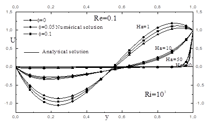
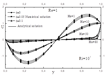
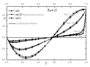
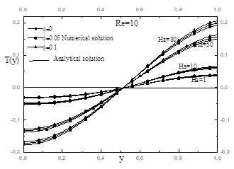
The horizontal velocity profiles show the presence of a single maximum value for all considered cases displayed in Figures 5-7, which testifies of the fact that the flow is unicellular and clockwise, mainly driven by the moving upper wall, signifying that the shear imposes a one-way flow. Whereas the temperature profile shows two zones with negative and positive signs, owing to the flow nature and the cooperative effects of the moving wall and buoyancy forces. The heat got into the left side of the enclosure, driven by the fluid near the upper section of the enclosure gets out by the right side of the cavity. Hence, the flow becomes cold and goes back near the inferior side of the cavity (y = 0). Explaining both regions of the temperature profile with signs (-, +) and this is independent of the concentration $\Phi$.
It was further observed that the concentration effect on temperature profiles and velocity, becomes increasingly insignificant when the Reynolds number increases, because the effect of viscosity caused by the addition of the ferroparticles is neutralized by the forced convection. As for Hartmann number it’s obvious that as Ha increases, the extremum values of temperature amplify testifying of the fact that the flow loses its intensity which can be confirmed from velocity profiles, where as Ha increases the fluid circulation becomes slower.
a)
b)
Figure 5. a) The horizontal velocity and b) temperature profiles at a mid-length of the cavity, along the vertical coordinate for coordinate for $A=16, R i=10^{3}, \operatorname{Re}=0.1$ for various values of $\Phi$ and various values of $H a$
a)
b)
Figure 6. a) The horizontal velocity and b) temperature profiles at a mid-length of the cavity, along the vertical coordinate for coordinate for $A=16, R i=10^{3}, \operatorname{Re}=1$ for various values of $\Phi$ and various values of $H a$
a)
b)
Figure 7. a) The horizontal velocity and b) temperature profiles at a mid-length of the cavity, along the vertical coordinate for coordinate for $A=16, R i=10^{3}, \operatorname{Re}=10$ for various values of $\Phi$ and various values of $\mathrm{Ha}$
5.3 Heat transfer rate
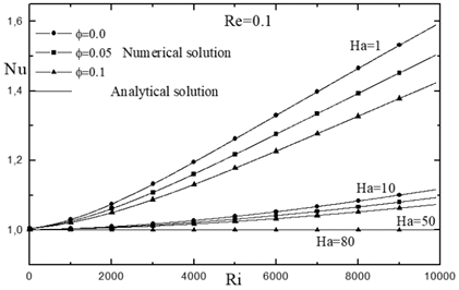
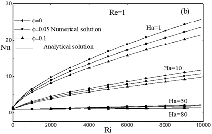
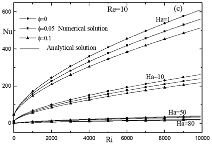
The evolution of the average Nusselt number, $\overline{N u}$, are reported, against $R i$, for Re given, each $H a$ and various $\Phi$, in Figures 8,9 and 10 , it is found that the heat transfer rate increases with $R i$, because increasing $R i$ increases the buoyancy effect causing the convection to become the driving force for movement. On the other hand, $\overline{N u}$ reduces when Hartmann number increases which agrees with earlier findings.
Figure 8. Evolution of the Nusselt number with $R i$ for $R e=0.1, A=16$ for various values of $\Phi$ and various values of $\mathrm{Ha}$
Figure 9. Evolution of the Nusselt number with $R i$ for $R e=1, A=16$ for various values of $\Phi$ and various values of $\mathrm{Ha}$
Figure 10. Evolution of the Nusselt number with $R i$ for $\operatorname{Re}=10, A=16$ for various values of $\Phi$ and various values of $\mathrm{Ha}$
where, increasing Hartmann number was proven to reduce the flow intensity within the enclosure. Moreover, increasing the concentration of ferroparticles decreases the heat transfer rate, $\overline{N u}$, despite that thermal conductivity of ferroparticles is great compared to that of the pure fluid. As can be seen, the curves that have high concentrations are always below the others that have low concentrations for a given $R e$. This can be explained by the increase in viscosity due to the increase in the concentration of ferroparticles, and the lengthening of the cavity.
On the other hand, these results show that heat transfer enhances with $R e$ as a beneficial result of the shear force on Nusselt number. In addition, an increase / (a decrease) of $R e$, implies that the heat transfer is governed by forced / (natural) convection.
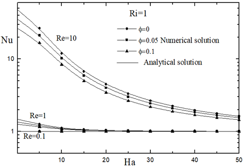
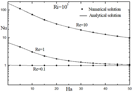
To further investigate how $H a$ affects heat transfer rate, we refer to Figures 11 and 12 , that portray changes in $\overline{N u}$ with Hartmann numbers at $R i=1$ and $R i=10^{3}$. Heat transfer rate shrinks fast up to $H a=20$. However, for larger Hartmann number $(H a \geq 40)$, the value of $\overline{N u}$ becomes more or less constant for ferrofluid. It's worth mentioning, that for a strong Ri number, the particle concentration has no effect on heat transfer, but for low values of $R i$, the effect of $\Phi$ becomes visible.
Figure 11. Evolution of the Nusselt number with $H a$ for $R i=1, A=16$ for various values of $\Phi$ and various values of $R e$
Figure 12. Evolution of the Nusselt number with $H a$ for $R i=10^{3}, A=16$ for various values of $\Phi$ and various values of $R e$
5.4 Flow intensity
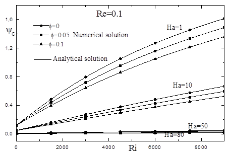
The evolution of $\Psi_{C}$ as reported, against $R i$, for $R e=0.1$, and various values of $H a$ and $\Phi$, is given in the Figure 13.
It is clear that increasing $H a$ leads to reducing the strength of the flow as shown by Figure 13 where $\psi_{c}$ decreases. Such phenomenon can be explained by the fact that higher Hartmann numbers induces magnetic field; as a result, Lorentz force acting on the flow domain is introduced. The said force plays the role of a magnetic viscosity lessening the intensity of the flow circulation within the cavity. Increasing Hartmann number $(H a=50, H a=80)$ strongly impacts ferrofluid compared to plain fluid owing to the presence of magnetic particles, causing it to be more vulnerable to magnetic fields.
Figure 13. Evolution of the stream function in the central part of the cavity, with $R i$ for $\operatorname{Re}=0.1$ and $A=16$ for various values of $\Phi$ and various values of $\mathrm{Ha}$
On the other hand, and for low values of $H a$, the fluid intensity increases with $R i$ as a beneficial effect of increasing the buoyancy force. On the other hand, increasing $\Phi$ slows the ferrofluid circulation, where increasing the concentration increases the viscosity; hence, reduce the flow intensity. The said effect of ferroparticles concentration becomes more pronounced as $R i$ increases causing natural convection to dominate the convective regime. As for high values of Hartman, $\Psi_{C}$ becomes practically constant and the effect of $\Phi$ vanishes as the magnetic viscosity induced by high values of $H a$ is more important compared to the viscosity caused by the ferroparticles concentration.
The present work investigates mixed convection within a closed shallow rectangular cavity (Aspect ratio A=16) occupied with a ferrofluid in the presence of a magnetic field, both analytically and numerically. Uniform density of heat fluxes is applied to short vertical walls, while the horizontal ones are adiabatic with the top wall sliding with a uniform velocity from left to right (i.e., the direction of applied heat fluxes).
The numerical solution is obtained using the well-known finite volume method to solve the governing equations. On the other hand, the parallel flow approximation, valid in the central region of the cavity is adopted for the analytical solution. Results were given for a wide range of controlling parameters, $\operatorname{Re}(0.1 \leq \operatorname{Re} \leq 10), R i\left(1 \leq R i \leq 10^{4}\right), H a(1 \leq H a \leq$ 80) and $\Phi(0 \leq \Phi \leq 0.1)$. The key findings can be listed as follows:
Given that most works in the field adopt a numerical approach, the analytical solution elaborated in the present work can be of importance, as it agrees perfectly with the numerical solution which testify the accuracy of both solutions and gives further authentication to the reached conclusions for the wide range of governing parameters. The present results are intended to clarify some inconsistencies between previous studies on ferrofluids in terms of heat transfer intensification and the role of magnetic field in the case of mixed convection, especially their capabilities for applications such as cooling systems.
|
A |
aspect ratio of the cavity $\left(L^{\prime} / H^{\prime}\right)$ |
|
B |
magnetic field (Tesla) |
|
C |
dimensionless temperature gradient in the x-direction |
|
$g$ |
gravitational acceleration $\left(\mathrm{m} / \mathrm{s}^{2}\right)$ |
|
$G r$ |
Grashof number |
|
$H^{\prime}$ |
height of the enclosure (m) |
|
$H a$ |
Hartmann number |
|
$h$ |
heat exchange coefficient $\left(W / m^{2} K\right)$ |
|
$k$ |
thermal conductivity of fluid $(W / m K)$ |
|
$\bar{k}$ |
dimensionless parameter, $\left[=k_{f f} / k_{f}\right]$ |
|
$L^{\prime}$ |
length of the rectangular enclosure (m) |
|
$Nu$ |
local Nusselt number |
|
$\frac{N u}{N u}$ |
average Nusselt number |
|
$P e$ |
Peclet number |
|
$P r$ |
Prandtl number |
|
$p$ |
Dimensionless pressure $\left[=p^{\prime} / \rho_{f} U_{0}^{\prime 2}\right]$ |
|
$q^{\prime}$ |
constant heat flux per unit area $\left(W / m^{2}\right)$ |
|
$R a$ |
Rayleigh number |
|
$R e$ |
Reynolds number |
|
$R i$ |
Richardson number |
|
$t$ |
dimensionless time, $\left[=t^{\prime} U_{0}^{\prime} / H^{\prime}\right]$ |
|
$T$ |
dimensionless temperature, $\left[=\left(T^{\prime}-T_{c}^{\prime}\right) / \Delta T^{*}\right]$ |
|
$T_{c}^{\prime}$ |
reference temperature at the geometric centre of the enclosure (K) |
|
$\Delta T^{*}$ |
characteristic temperature $\left[=q^{\prime} H^{\prime} / k_{f}\right]$ (K) |
|
$(u, v)$ |
dimensionless velocity components $\left[=\left(u^{\prime}, v^{\prime}\right) / U_{0}^{\prime}\right]$ |
|
$U_{0}^{\prime}$ |
lid-velocity $(\mathrm{m} / \mathrm{s})$ |
|
$(x, y)$ |
dimensionless coordinates $\left[=\left(x^{\prime}, y^{\prime}\right) / H^{\prime}\right]$ |
|
Greek symbols |
|
|
$\alpha$ |
thermal diffusivity $\left(\mathrm{m}^{2} / \mathrm{s}\right)$ |
|
$\bar{\alpha}$ |
dimensionless parameter, $\left[=\alpha_{f f} / \alpha_{f}\right]$ |
|
$\beta$ |
thermal expansion coefficient $(1 / K)$ |
|
$\bar{\beta}$ |
dimensionless parameter, $\left[=\left(\rho \beta^{\prime}\right)_{f f} /\left(\rho \beta^{\prime}\right)_{f}\right]$ |
|
$v$ |
kinematic viscosity $\left(\mathrm{m}^{2} / \mathrm{s}\right)$ |
|
$\bar{v}$ |
dimensionless parameter, $\left[=v_{f f} / v_{f}\right]$ |
|
$\mu$ |
dynamic viscosity $(\mathrm{Pa} \cdot s)$ |
|
$\rho$ |
density of base fluid $\left(\mathrm{kg} / \mathrm{m}^{3}\right)$ |
|
$\sigma_{f f}$ |
dimensionless conductivity of ferrofluid |
|
$\bar{\sigma}$ |
conductivity of ferrofluid |
|
$\Phi$ |
ferroparticle volume fraction |
|
$\psi$ |
dimensionless stream function, $\left[=\psi^{\prime} / \alpha_{f}\right]$ |
|
$\Omega$ |
dimensionless parameter, $[=\bar{\beta} /(\bar{\rho} \bar{v} \bar{\alpha})]$ |
|
Superscripts |
|
|
' |
dimensional variable |
|
Subscripts |
|
|
c |
value relative to the centre of the enclosure or critical value |
|
f |
base fluid |
|
m |
minimum value |
|
ff |
ferrofluid |
|
fp |
ferroparticle |
[1] Philip, J.P., Shima, D., Raj, B. (2007). Enhancement of thermal conductivity in magnetite based nanofluid due to chainlike structures. Appl. Phys. Lett., 91(20): 203108. https://doi.org/10.1063/1.2812699
[2] Gavili, A., Zabihi, F., Isfahani, T.D. Sabbaghzadeh, J. (2012). The thermal conductivity of water base ferrofluids under magnetic field. Exp. Therm. Fluid Sci., 41: 94-98. https://doi.org/10.1016/j.expthermflusci.2012.03.016
[3] Lajvardi, M., Moghimi-Rad, J., Hadi, I., Gavili, A., Dallali Isfahani, T., Zabihi, F., Sabbaghzadeh, J. (2010). Experimental investigation for enhanced ferrofluid heat transfer under magnetic field effect. Journal of Magnetism and Magnetic Materials, 322(21): 3508-3513. https://doi.org/10.1016/j.jmmm.2010.06.054
[4] Nkurikiyimfura, I., Wang, Y., Pan, Z. (2013). Heat transfer enhancement by magnetic nanofluids-A review. Renewable and Sustainable Energy Reviews, 21: 548-561. https://doi.org/10.1016/j.rser.2012.12.039
[5] Rudraiah, N., Barron, R.M., Venkatachalappa M. Subbaraya, C.K. (1995). Effect of a magnetic field on free convection in a rectangular enclosure. International Journal of Engineering Science, 33(8): 1075-1084. https://doi.org/10.1016/0020-7225(94)00120-9
[6] Jafari, A., Tynjälä, T., Mousavi, S. M., Sarkomaa, P. (2008). Simulation of heat transfer in a ferrofluid using computational fluid dynamics technique. International Journal of Heat and Fluid Flow, 29(4): 1197-1202. https://doi.org/10.1016/j.ijheatfluidflow.2008.01.007
[7] Khanafer, K., Vafai, K., Lightstone, M. (2003). Buoyancy-driven heat transfer enhancement in a two-dimensional enclosure utilizing nanofluids. International Journal of Heat and Mass Transfer, 46(19): 3639-3653. https://doi.org/10.1016/S0017-9310(03)00156-X
[8] Yamaguchi, H., Niu, X. D., Zhang, X. R., Yoshikawa, K. (2009). Experimental and numerical investigation of natural convection of magnetic fluids in a cubic cavity. Journal of Magnetism and Magnetic Materials, 321(22): 3665-3670. https://doi.org/10.1016/j.jmmm.2009.07.013
[9] Mehrez, Z., El Cafsi, A. (2021). Heat exchange enhancement of ferrofluid flow into rectangular channel in the presence of a magnetic field. Applied Mathematics and Computation, 391: 125634. https://doi.org/10.1016/j.amc.2020.125634
[10] Sheikholeslami, M., Vajravelu, K.J.A.M. (2017). Nanofluid flow and heat transfer in a cavity with variable magnetic field. Applied Mathematics and Computation, 298: 272-282. https://doi.org/10.1016/j.amc.2016.11.025
[11] Szabo, P.S., Früh, W.G. (2018). The transition from natural convection to thermomagnetic convection of a magnetic fluid in a non-uniform magnetic field. Journal of Magnetism and Magnetic Materials, 447: 116-123. https://doi.org/10.1016/j.jmmm.2017.09.028
[12] Yamaguchi, H., Kobori, I., Uehata, Y. (1999). Heat transfer in natural convection of magnetic fluids. Journal of Thermophysics and Heat Transfer, 13(4): 501-507. https://doi.org/10.2514/2.6468
[13] Cheng, Y., Li, D. (2019). Experimental investigation on convection heat transfer characteristics of ferrofluid in a horizontal channel under a non-uniform magnetic field. Applied Thermal Engineering, 163: 114306. https://doi.org/10.1016/j.applthermaleng.2019.114306
[14] Bian, W., Vasseur, P., Bilgen, E., Meng, F. (1996). Effect of an electromagnetic field on natural convection in an inclined porous layer. International Journal of Heat and Fluid Flow, 17(1): 36-44. https://doi.org/10.1016/0142-727X(95)00070-7
[15] Aminfar, H., Mohammad Pourfard, M., Zonouzi, S.A. (2013). Numerical study of the ferrofluid flow and heat transfer through a rectangular duct in the presence of a non-uniform transverse magnetic field. J. Magn. Magn. Mater., 327: 31-42. https://doi.org/10.1016/j.jmmm.2012.09.011
[16] Ashouri, M., Ebrahimi, B., Shafii, M.B., Saidi, M.H., Saidi, M.S. (2010). Correlation for Nusselt number in pure magnetic convection ferrofluid flow in a square cavity by a numerical investigation. J. Magn. Magn. Mater., 322: 3607-3613. https://doi.org/10.1016/j.jmmm.2010.05.041
[17] Jue, T.C. (2006). Analysis of combined thermal and magnetic convection ferrofluid flow in a cavity. Int. Commun. Heat Mass Transfer, 33: 846-852. https://doi.org/10.1016/j.icheatmasstransfer.2006.02.001
[18] Kefayati, G.H.R. (2014). Natural convection of ferrofluid in a linearly heated cavity utilizing LBM. J. Mol. Liq., 191: 1-9. https://doi.org/10.1016/j.molliq.2013.11.021
[19] Mohsen, S. Mofid, G.B. (2014). Free convection of ferrofluid in a cavity heated from below in the presence of an external magnetic field. Powder Technol., 256: 490-498. https://doi.org/10.1016/j.powtec.2014.01.079
[20] Mojumder, S., Saha, S.O., Saha, S., Mamun, M.A.H. (2015). Effect of magnetic field on natural convection in a C-shaped cavity filled with ferrofluid. Procedia Engineering, 105(96): 104. https://doi.org/10.1016/j.proeng.2015.05.012
[21] Nahak, M.P., Triveni, M.K., Panua, R. (2017). Numerical investigation of mixed convection in a lid-driven triangular cavity with a circular cylinder using ANN modeling. International Journal of Heat and Technology, 35(4): 903-918. https://doi.org/10.18280/ijht.350427
[22] Tiwari, R.K., Das, M.K. (2007). Heat transfer augmentation in a two-sided lid-driven differentially heated square cavity utilizing nanofluids. International Journal of Heat and Mass Transfer, 50(9-10): 2002-2018. https://doi.org/10.1016/j.ijheatmasstransfer.2006.09.034
[23] Abdelkhalek, M.M. (2008). Mixed convection in a square cavity by a perturbation technique. Computational Materials Science, 42(2): 212-219. https://doi.org/10.1016/j.commatsci.2007.07.004
[24] Abu-Nada, E., Chamkha, A.J. (2010). Mixed convection flow in a lid-driven inclined square enclosure filled with a nanofluid. European Journal of Mechanics-B/Fluids, 29(6): 472-482. https://doi.org/10.1016/j.euromechflu.2010.06.008
[25] Mahmoodi, M. (2011). Mixed convection inside nanofluid filled rectangular enclosures with moving bottom wall. Thermal Science, 15(3): 889-903. https://doi.org/10.2298/TSCI101129030M
[26] Gibanov, N.S., Sheremet, M.A., Oztop, H.F., Abu-Hamdeh, N. (2017). Effect of uniform inclined magnetic field on mixed convection in a lid-driven cavity having a horizontal porous layer saturated with a ferrofluid. International Journal of Heat and Mass Transfer, 114: 1086-1097. https://doi.org/10.1016/j.ijheatmasstransfer.2017.07.001
[27] Hekmat, M.H., Ziarati, K.K. (2019). Effects of nanoparticles volume fraction and magnetic field gradient on the mixed convection of a ferrofluid in the annulus between vertical concentric cylinders. Applied Thermal Engineering, 152: 844-857. https://doi.org/10.1016/j.applthermaleng.2019.02.124
[28] Job, V.M., Gunakala, S.R. (2018). Mixed convective ferrofluid flow through a corrugated channel with wall-mounted porous blocks under an alternating magnetic field. International Journal of Mechanical Sciences, 144: 357-381. https://doi.org/10.1016/j.ijmecsci.2018.05.054
[29] Mehmood, Z. (2019). Numerical simulations and linear stability analysis of mixed thermomagnetic convection through two lid-driven entrapped trapezoidal cavities enclosing ferrofluid saturated porous medium. International Communications in Heat and Mass Transfer, 109: 104345. https://doi.org/10.1016/j.icheatmasstransfer.2019.104345
[30] Sheikholeslami, M., Chamkha, A.J. (2016). Flow and convective heat transfer of a ferro-nanofluid in a double-sided lid-driven cavity with a wavy wall in the presence of a variable magnetic field. Numerical Heat Transfer, Part A: Applications, 69(10): 1186-1200. https://doi.org/10.1080/10407782.2015.1125709
[31] Yu, W., France, D.M., Choi, S.U., Routbort, J.L. (2007). Review and assessment of nanofluid technology for transportation and other applications. United States. ANL/ESD/07-9. https://doi.org/10.2172/919327
[32] Maxwell, J.C. (1904). A Treatise on Electricity and Magnetism. Second ed., Oxford University Press, Cambridge: 435-441.
[33] Corcione, M. (2010). Heat transfer features of buoyancy-driven nanofluids inside rectangular enclosures differentially heated at the sidewalls. International Journal of Thermal Sciences, 49(9): 1536-1546. https://doi.org/10.1016/j.ijthermalsci.2010.05.005
[34] Lamsaadi, M., Naimi, M., Hasnaoui, M. (2006). Natural convection heat transfer in shallow horizontal rectangular enclosures uniformly heated from the side and filled with non-Newtonian power law fluids. Energy conversion and Management, 47(15-16): 2535-2551. https://doi.org/10.1016/j.enconman.2005.10.028
[35] Patankar, S.V. (1980). Numerical Heat Transfer and Fluid Flow. Hemisphere, Washington DC. CRC press.
[36] Bejan, A. (1983). The boundary layer regime in a porous layer with uniform heat flux from the side. International Journal of Heat and Mass Transfer, 26(9): 1339-1346. https://doi.org/10.1016/S0017-9310(83)80065-9