Yap Yit Fatt* | Afshin Goharzadeh
© 2021 IIETA. This article is published by IIETA and is licensed under the CC BY 4.0 license (http://creativecommons.org/licenses/by/4.0/).
OPEN ACCESS
Particle deposition occurs in many engineering multiphase flows. A model for particle deposition in two-fluid flow is presented in this article. The two immiscible fluids with one carrying particles are model using incompressible Navier-Stokes equations. Particles are assumed to deposit onto surfaces as a first order reaction. The evolving interfaces: fluid-fluid interface and fluid-deposit front, are captured using the level-set method. A finite volume method is employed to solve the governing conservation equations. Model verifications are made against limiting cases with known solutions. The model is then used to investigate particle deposition in a stratified two-fluid flow and a cavity with a rising bubble. For a stratified two-fluid flow, deposition occurs more rapidly for a higher Damkholer number but a lower viscosity ratio (fluid without particle to that with particles). For a cavity with a rising bubble, deposition is faster for a higher Damkholer number and a higher initial particle concentration, but is less affected by viscosity ratio.
two-fluid flow, particle deposition, level-set method
In many engineering flows involving particles, the particles deposit on surfaces. For examples, deposition of wax, hydrates and asphaltene in pipelines and fouling in heat exchangers. Formation of deposit reduces flow, increases pressure drop and possibly clogs flow passages. Cleaning of flow passages requires additional cost and usually involves temporary operation shutdown. Often, particles carried in multiphase flows deposit as well for example oil-water-gas mixture in pipelines and water-steam mixture in heat exchangers. To overcome such a problem, understandings of the underlying physics for particle deposition in multiphase flow and its prediction are required.
Particle deposition in a single-fluid flow has been modeled for wax [1], hydrates [2] and asphaltene [3] deposition in pipelines, fouling in heat exchangers [4-6], super conformal electrodeposition in semiconductor manufacturing technology [7], chemical vapor deposition [8], combined deposition-etching-lithography processes in integrated circuits fabrication [9] and laser deposition involving phase change [10]. Within a single-fluid flow environment, a particle deposition modeling framework has generally four components. These are to (1) determine the flow fields (fluid transport), (2) calculate the particle distribution (particle transport), (3) model the sticking of particles onto the fluid-deposit front (particle deposition) and (4) evolve the fluid-deposit interface (capturing fluid-deposit front).
The flow field can be conveniently described using for example the Navier-Stokes equations for Newtonian fluids or more generally the Cauchy momentum equation coupled with appropriate constitutive relations for non-Newtonian fluids.
The transport of particles can be driven by inertia, Brownian diffusion, thermophoresis, diffusiophoresis, etc. Its temporal distribution can be determined using a Lagrangian or an Eulerian framework. In the Lagrangian framework, a large number of particles are tracked individually by integrating their respective momentum equation [11]. Whereas in an Eulerian framework, particle distribution is determined in terms of concentration via mass conservation equation [12-14] or/and momentum conservation [15-17].
Particle deposition onto the fluid-deposit front can be modeled via a critical length with a sticking probability [18]. Basically, a particle will probabilistically deposit onto the fluid-deposit front if its distance from the effective roughness height of fluid-deposit front is equal or less than half of the particle's diameter [19, 20]. In many studies, a unity sticking probability is assumed [21, 22]. This approach is more suited to Lagrangian description of particle transport. For Eulerian description of particle transport, an m-th order deposition reaction [23-25] can be conveniently used. Asphaltene particle deposition [23], SiO2 deposition [26] and copper electrodeposition [27] have been modeled as first order reaction. Besides, experimentally developed empirical correlations for modeling of particle deposition has been proposed and employed [28].
To treat the fluid-deposit front, either a front-tracking approach [29, 30] or a front-capturing approach, e.g., the VOF [31], level-set [32], enthalpy–porosity [33] and total concentration [34] approaches can be employed. For a thin deposit layer compared to the characteristic length, a static fluid-deposit front is assumed. This avoids the difficulty of tracking/capturing the fluid-deposit front.
There exists only one moving interface, i.e., fluid-deposit front, for deposition in single-fluid flow environment. However, for particle deposition in multi-fluid flow environment, there are additional dynamic fluid-fluid interfaces that can easily undergo topological changes. Therefore, apart from the above mentioned four components of the modeling framework, one additional component is needed to evolve the fluid-fluid interfaces. The fluid-fluid interface can be captured for example using the level-set, VOF [35-37] and coupled level-set VOF [38] approach. The framework now has to address two or more moving interfaces and simultaneously couple the multi-fluid flow (velocity and pressure), concentration and temperature fields via appropriately enforced interfacial conditions at the interfaces. Modeling work then becomes challenging.
Notable numerical investigation for deposition in multi-fluid flow environment is that of Huang et al. [39]. They presented a model for wax deposition in two-dimensional stratified oil-water flow. The study shows the need to consider the movement of the oil-water interface to produce a more accurate prediction. This is not considered in previous studies. For this unidirectional flow, the interface is simple and amenable to an analytical solution. Although works well for stratified flow with simple interface, this approach is difficult to be extended to more general flows. Ramirez-Jaramillo et al. [40] studied deposition of asphaltene particles in a four-phase oil-gas-water-asphaltene flow in pipe. The flow is determined from empirical relations, without any fluid-fluid interface tracked or captured. The deposit profile is then determined by accounting for the mass of asphaltene particles deposited. Van Parys et al. [41] modeled the mass transport in electro-deposition process. The small gas bubbles formed in the process (another fluid) are tracked using a Langrangian approach. From the article, it is not clear if the movement of fluid-deposit front on the electrode is accounted for.
After extensive literature searches, it is concluded that numerical modeling of such a multiphase flow deposition process is very scarcely reported in existing literatures. Therefore, it is explored here in this article. Specifically, this study focuses on the numerical modeling framework for particle deposition in a two-fluid environment where fluids are immiscible with particles carried by one of the fluids.
In the following five sections of the article, problem description, mathematical formulation, solution procedure, results and conclusions are presented sequentially.
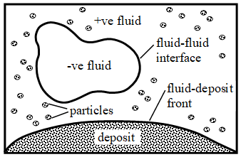
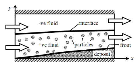
The domain of interest is shown in Figure 1. There are three regions: +ve fluid, -ve fluid and deposit. The two fluids are immiscible. There are two interfaces: fluid-fluid interface and fluid-deposit front. Particles are carried by +ve fluid. These particles however do not convect or diffuse into the -ve fluid. The particles deposit gradually onto the front and the impermeable rigid solid deposit layer grows with time. The movement of both interface and front are strongly coupled to the underlying fluid flow and deposition process. Therefore, they are not known in advanced and emerge as part of the solution.
Figure 1. Domain with two fluids and a deposit
3.1 Capturing the fluid-fluid interface
A level-set function [42] is used to represent the fluid-fluid interface via
${{\varphi }_{f}}\equiv \left\{ \begin{array}{*{35}{l}} +{{d}_{f}}, \\ 0, \\ -{{d}_{f}}, \\\end{array}\begin{matrix} {} \\\end{matrix}\begin{array}{*{35}{l}} \text{in }+\text{ve fluid} \\ \text{at interface} \\ \text{otherwise} \\\end{array} \right.$ (1)
where, df is the shortest distance from the fluid-fluid interface. The movement of fluid-fluid interface is captured via
$\frac{\partial {{\phi }_{f}}}{\partial t}+\vec{u}\bullet \nabla {{\phi }_{f}}=0,\text{ at interface}$ (2)
where, $\vec{u}$ is the fluid velocity. Redistancing is performed [43, 44] after advection with Eq. (2) to maintain ϕf as a distance function, i.e., $\left|\nabla \phi_{f}\right|=1$. Besides, to minimize mass loss/gain, global [45] or local [46] mass correction is incorporated.
3.2 Capturing the fluid-deposit front
Another level-set function is used to represent the fluid-deposit front via
${{\varphi }_{d}}\equiv \left\{ \begin{array}{*{35}{l}} +{{d}_{d}}, \\ 0, \\ -{{d}_{d}}, \\\end{array}\begin{matrix} {} \\\end{matrix}\begin{array}{*{35}{l}} \text{in deposit} \\ \text{at front} \\ \text{otherwise} \\\end{array} \right.$ (3)
where, dd is the shortest distance from the fluid-deposit front. The movement of the fluid-deposit front is captured via
$\frac{\partial {{\phi }_{d}}}{\partial t}+{{\vec{u}}_{d,ext}}\bullet \nabla {{\phi }_{d}}=0,\text{ at front}$ (4)
where, $\vec{u}_{d, e x t}$ is a normally extended velocity field of the fluid-deposit front $\vec{u}_{d}$ with the following property maintained.
${{\vec{u}}_{d,ext}}={{\vec{u}}_{d}},\text{ at front}$ (5)
This extension can be performed via the method in [47].
3.3 Particle deposition
The particle deposition process at the fluid-deposit front is assumed to be a first order reaction. The particle deposition flux can be expressed as
$\vec{q}=-{{\rho }_{d}}{{\vec{u}}_{d}}=kC{{\hat{n}}_{d}},\text{ at front}$ (6)
where, ρd, k, C and $\hat{n}_{d}$ are the density of the deposit, the deposition reaction rate, the particle concentration and unit normal vector pointing out of the fluid region into the deposit region respectively. The velocity of the fluid-deposit front can then be written as
${{\vec{u}}_{d}}=-\frac{kC{{{\hat{n}}}_{d}}}{{{\rho }_{d}}},\text{ at front}$ (7)
3.4 Particle transport
Transport of the particles for the whole domain is governed by
$\frac{\partial C}{\partial t}+\nabla \bullet (\vec{u}C)=\nabla \bullet (D\nabla C)-kC\delta ({{\varphi }_{d}}+\varepsilon )\left| \nabla {{\varphi }_{d}} \right|$ (8)
where, D and δ are respectively the diffusion coefficient and a smoothed Dirac delta function over a width of 2ε. The Dirac delta function can be approximate as
$\delta (\varphi )=\left\{ \begin{array}{*{35}{l}} \frac{1+\cos (\pi \varphi /\varepsilon )}{2\varepsilon }, \\ 0, \\\end{array} \right.\begin{matrix} {} \\\end{matrix}\begin{array}{*{35}{l}} \text{if }\left| \varphi \right|<\varepsilon \\ \text{otherwise} \\\end{array}$ (9)
and the diffusion coefficient can be evaluated as
$D({{\varphi }_{f}},{{\varphi }_{d}})=\left\{ \begin{array}{*{35}{l}} D, \\ 0, \\\end{array}\begin{matrix} {} \\\end{matrix}\begin{array}{*{35}{l}} \text{if }{{\varphi }_{f}}>0\text{ and }{{\varphi }_{d}}<0 \\ \text{else} \\\end{array} \right.$ (10)
In the numerical solution of Eqns. (4) and (8), particles can drift into the -ve fluid or trapped within the deposit. These particles are redistributed into the all the control volumes (CVs) of +ve fluid evenly using the particle correction approach in [32].
3.5 Fluid transport
Within a unified formulation, the transport of the +ve and -ve fluids is coupled and governed by
$\nabla \bullet \vec{u}=0$ (11)
$\begin{align} & \frac{\partial (\rho \vec{u})}{\partial t}+\nabla \bullet (\rho \vec{u}\vec{u})=-\nabla p+\nabla \bullet \left[ \mu (\nabla \vec{u}+\nabla {{{\vec{u}}}^{T}}) \right] \\ & \begin{matrix} {} & {} & {} & {} \\\end{matrix}\begin{matrix} {} & {} \\\end{matrix}\begin{matrix} {} & {} \\\end{matrix}+\rho \vec{g}-(\nabla \bullet {{{\hat{n}}}_{f}})\sigma {{{\hat{n}}}_{f}}\delta ({{\varphi }_{f}}) \\\end{align}$ (12)
where, ρ, μ and σ are respectively the fluid density, viscosity and surface tension. In Eq. (12), $p, \vec{g}$ and $\hat{n}_{f}$ are respectively pressure, gravitational acceleration and unit normal vector of the fluid-fluid interface pointing from the -ve fluid into the +ve fluid. The last term in Eq. (12) models the effect of surface tension via Continuum Surface Force Model [48]. The density and viscosity can be evaluated respectively as
$\rho ({{\varphi }_{f}},{{\varphi }_{d}})=\left\{ \begin{array}{*{35}{l}} \left( 1-H({{\varphi }_{f}}) \right){{\rho }_{-}}+H({{\varphi }_{f}}){{\rho }_{+}},\text{ if }{{\varphi }_{d}}\le 0 \\ {{\rho }_{d}}\begin{matrix} {} & {} & \begin{matrix} {} \\\end{matrix}\begin{matrix} {} & {} & {} \\\end{matrix}\begin{matrix} {} & {} \\\end{matrix}\text{, if }{{\varphi }_{d}}>0 \\\end{matrix} \\\end{array} \right.$ (13)
$\mu ({{\varphi }_{f}},{{\varphi }_{d}})\begin{matrix} {} \\\end{matrix}\left\{ \begin{array}{*{35}{l}} \frac{1}{\mu }=\frac{1-H({{\varphi }_{f}})}{{{\mu }_{-}}}+\frac{H({{\varphi }_{f}})}{{{\mu }_{+}}},\text{ if }{{\varphi }_{d}}\le 0 \\ \mu =\infty \begin{matrix} {} & {} & \begin{matrix} {} \\\end{matrix}\begin{matrix} {} & {} & {} \\\end{matrix}\begin{matrix} {} \\\end{matrix}\text{, if }{{\varphi }_{d}}>0 \\\end{matrix} \\\end{array} \right.$ (14)
where, the smoothed Heaviside function is approximated as
$H(\varphi )=\left\{ \begin{array}{*{35}{l}} 0, \\ \frac{\varphi +\varepsilon }{2\varepsilon }+\frac{1}{2\pi }\sin \left( \frac{\pi \varphi }{\varepsilon } \right), \\ 1, \\\end{array}\begin{matrix} {} \\\end{matrix}\begin{array}{*{35}{l}} \text{if }\varphi <-\varepsilon \\ \text{if }\left| \varphi \right|\le \varepsilon \\ \text{if }\varphi >+\varepsilon \\\end{array} \right.$ (15)
The conservation equations (Eqns. (8), (11) and (12)) can be represented as a generic transient convection-diffusion equation. The finite volume method [49, 50] is used to solve this generic equation. The convective and diffusive terms are treated respectively using 2nd order upwind scheme with SUPERBEE limiter [51] and 2nd order central differencing scheme. Time integration is performed using a fully implicit scheme. The SIMPLER algorithm is used to couple the velocity and pressure. The level-set equations (Eqns. (2) and (4)) are spatially discretized with WENO5 [52] and temporally integrated using TVD-RK2 [53] within a narrow-band framework [44]. The solution procedure is as follows:
(1) Specify the initial conditions (i.e., t=0) of ϕf, ϕd, $\vec{u}$, p and C.
(2) Advance the time step to t+Δt.
(3) Solve Eq. (2) for $\left.\phi_{f}\right|^{t+\Delta t}$.
(4) Solve Eq. (4) for $\left.\phi_{d}\right|^{t+\Delta t}$.
(5) Solve Eqns. (11) and (12) for $\left.\vec{u}\right|^{t+\Delta t}$ and $\left.p\right|^{t+\Delta t}$ using the SIMPLER algorithm.
(6) Solve Eq. (8) for $\left.C\right|^{t+\Delta t}$.
(7) Repeat steps (3) to (6) until the solution converges.
(8) Perform particle redistribution [32].
(9) Perform global [45] or local [46] mass correction.
(10) Repeat steps (2) to (9) for all time steps.
Non-dimensionalization is performed using dimensionless quantities of time $t^{*}=t u_{o} / L$, coordinates $\vec{x}^{*}=\vec{x} / L$, velocities $\vec{u}^{*}=\vec{u} / u_{o} \quad, \quad$ pressure $\quad p^{*}=p / \rho_{+} u_{o}^{2} \quad$ and concentration $C^{*}=C / \rho_{d}$. In these definitions, $L$ and $u_{o}$ are the characteristic length and velocity respectively. Then, the current problem is governed by the following dimensionless parameters: fluid-fluid density ratio $\rho_{-} / \rho_{+}$, deposit-fluid density ratio $\rho_{d} / \rho_{+}$, viscosity ratio $\mu_{-} / \mu_{+}$, Reynolds number $R e=\rho_{+} u_{o} L / \mu_{+}$, Froude number $F r=u_{o} / \sqrt{g L}$, Weber number $W e=\rho_{+} u_{o}^{2} L / \sigma$, dimensionless initial particle concentration $C_{o}^{*}=C_{o} / \rho_{d}$, Peclet number $P e=u_{o} L / D$ and Damkohler number $D a=k L / D$. It should be mentioned that for the present study, the particle density and the deposit density are identical to that of the $+$ ve fluid, i.e., $\rho_{d} / \rho_{+}=1$. Therefore, no shrinkage occurs in the deposition process. Besides these dimensionless numbers, additional problem specific dimensionless numbers will be introduced when required.
5.1 Verification-bubble rising in a partially-filled container
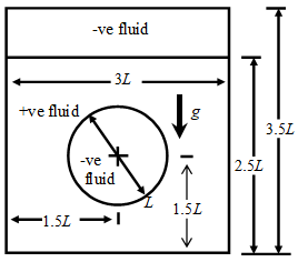
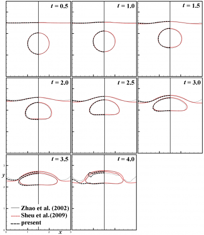
The schematic of an initially quiescent bubble rising in a partially filled container is shown in Figure 2. The bubble diameter L=1.0 is the characteristic length. The bubble rises and deforms the free interface in the process. The characteristic velocity is $u_{o}=\sqrt{g L}$. At both lower and upper walls, no-slip condition is applied. For the two side walls, free-slip is enforced. For this verification exercise, the dimensionless parameters are set to $\rho_{-} / \rho_{+}=0.5, \mu_{-} / \mu_{+}=0.5, \mathrm{Re}=200, F r=1$ and $W e=10$. Figure 3 shows the present and refs. [54, 55] solutions. The present solution agrees well with these existing solutions. This verifies implementation of the fluid-fluid interface capturing procedure. Note that the fluid-deposit front capturing procedure is temporarily turned off in this exercise.
Figure 2. A bubble rising in a partially-filled container
Figure 3. Fluid-fluid interfaces for a bubble rising in a partially-filled container
5.2 Verification-single-fluid flow in a channel with particle deposition
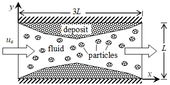
In Figure 4, particles are carried by a fluid into an initially clean channel. These particles deposit gradually onto the walls of the channel, and develops a deposit layer. The deposit layer is impermeable to fluid flow and changes the flow fields. Therefore the flow fields and the particle concentration field are strongly coupled. Given the symmetry of the problem, solution for the lower half of the domain is considered. Initially, there is no flow and no deposit in the channel. At the inlet of $x^{*}=0$, the following is enforced.
$u^{*}=1, v^{*}=0$, $C^{*}=\left\{\begin{array}{cl}0.1 & , 0.25 \leq y^{*} \leq 0.5 \\ 0 & , \text { otherwise }\end{array}\right.$ (16)
No slip condition is applied at the lower wall. Symmetric condition is applied at the middle symmetric plane.
The grid independent solution obtained on a mesh of 240×40 CVs with $\Delta t^{*}=5 \times 10^{-3}$ for the case of Re=1, $C_{o}^{*}=0.1$ Pe=15 and Da=10 is shown in Figure 5. The present solution is in good agreement with that of [34]. As the particle concentration is higher near the inlet, a thicker deposit develops. Along the channel, as particles are deposited, particle concentration decreases leading to an increasingly thinner deposit layer downstream. This exercise verifies implementation of the fluid-deposit front capturing procedure. Of course, the fluid-fluid interface capturing procedure is temporarily turned off.
Figure 4. Schematic of a single-fluid flow in a channel with particle deposition
Figure 5. Fluid-deposit front for Re=1, $C_{o}^{*}=0.1$ Pe=15 and Da=10
5.3 Particle deposition in a stratified two-fluid flow
Figure 6 shows a schematic of a channel with two stratified flowing fluid layers. The channel is initially clean (without deposit). With the height used as the characteristic length L, the channel has a dimensionless length of 3. At the inlet, both fluids have the same uniform velocity. The +ve fluid carries particles that deposit on lower wall and form a solid deposit layer. The deposit layer grows with time and because it is impermeable to fluid flow, the flow of the two fluids is affected. This in turn modifies the deposition process itself.
Figure 6. Schematic of particle deposition in a stratified two-fluid flow
The solution of a standard case will be first presented. The effect of various governing dimensionless numbers will then be investigated by comparison with this standard case. For the standard case, $\rho_{-} / \rho_{+}=1.1, \mu_{-} / \mu_{+}=0.1, R e=1, F r=\infty$ (no gravitational effect), $W e=10, P e=15$ and $D a=10 .$ For stratified flow, the dimensionless thickness of $+$ ve fluid at the inlet, i.e., $h_{+} / L$, is required to fully specify the problem. It is set to $h_{+} / L=0.5$. The following initial and boundary conditions are enforced.
Initial conditions:
$\vec{u}^{*}=\overrightarrow{0}, C^{*}=0$ for $0 \leq x^{*} \leq 3$ and $0 \leq y^{*} \leq 1$ (17a)
Boundary Conditions
At the inlet $\left(x^{*}=0\right)$$u^{*}=1, v^{*}=0, \quad C^{*}= \begin{cases}0.1 & , 0.25 \leq y^{*} \leq 0.5 \\ 0 & , \text { otherwise }\end{cases}$ (17b)
At the outlet $\left(x^{*}=3\right)$$\frac{\partial u^{*}}{\partial x^{*}}=0 \quad, v^{*}=0, \quad \frac{\partial C^{*}}{\partial x^{*}}=0$ (17c)
At the upper and lower walls ( $y^{*}=0$ )$\vec{u}^{*}=\overrightarrow{0}, \frac{\partial C^{*}}{\partial y^{*}}=0$ (17d)
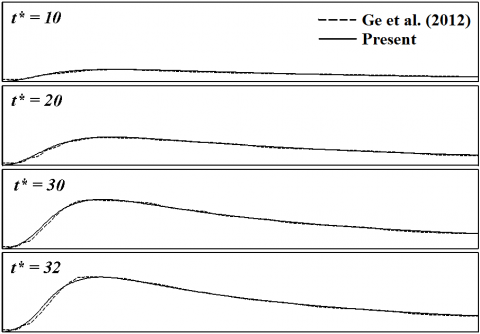
The fluid-fluid interface and fluid-deposit front obtained on different meshes are plotted in Figure 7a. A mesh of 40×80 CVs with $\Delta t *=2.5 \times 10^{-3}$ can generally resolve most of the important features of the solution. Therefore, this mesh size will be used in subsequent computations.
A more detailed evolution of both interface and front with velocity field superimposed for this standard case (Da=10) is given in Figure 8. The thickest deposit layer forms near the inlet where particles are constantly supplied from the in-flowing +ve fluid and thus the concentration is much higher. Generally as the deposit layer grows thicker over time, the average velocity of both fluid layers increase as the cross-sectional area for flow decreases.
Shown in Figure 7b is the interface and front for the case without particle deposition, i.e., Da=0. Of course, the front does not evolve over time and therefore is static. The flow of the two fluids reaches steady-state in a very short time, i.e., well before t*=8, and after which the fluid-fluid interface remains stationary. As such, the velocity field is included for completeness without overcrowding the figure. Comparison of the standard case in Figure 8 with Figure 7b reveals, as expected, that the formation of the deposit layer affects the flow significantly.
Figure 7. Fluid-fluid interface and fluid-deposit front at t*=0, 8, 16, 24, 32 and 40
Figure 8. The effect of Da at t*=8, 16, 24, 32 and 40
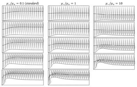
Figure 9. The effect of $\mu_{-} / \mu_{+}$ at $t *=8,16,24,32$ and 40
The Damkholer number of the standard case is now varied. It is progressively decreased from Da=10 to Da=5 and finally to Da=1. The results for these cases are shown in Figure 8. Generally, the amount of deposit formed up to a given time decreases with a lower Da, resulting in a much thinner deposit layer. Besides, for small Da, the thickness of the deposit layer downstream tends to be more uniform as particle concentration at the front is more uniform. The deposition process is increasingly dictated by the deposition reaction rather than diffusion. Even if there are particles at the front, most of them do not get deposited because of a low deposition reaction rate k, and will just be transported downstream.
Again, based on the standard case, the viscosity ratio $\mu_{-} / \mu_{+}$ is varied to investigate its effect while the other dimensionless parameters remain fixed. The viscosity ratio is increased from $\mu_{-} / \mu_{+}=0.1($ standard $)$ to $\mu_{-} / \mu_{+}=1$ and finally to $\mu_{-} / \mu_{+}$, spanning two orders of magnitude. Increase in $\mu_{-} / \mu_{+}$ implies the -ve fluid becomes relatively more viscous than the +ve fluid. With this, the -ve fluid flows generally slower and the -ve fluid layer becomes thicker constraint by mass conservation. This thicker -ve fluid layer squeezes the +ve fluid into a thinner layer, as clearly shown in Figure 9 at t*=8. This effectively concentrates the particles in the +ve fluid layer, increases particle transport to the fluid-deposit front and results in a higher particle concentration near the fluid-deposit front. Although governed by the same deposition kinetics, the deposit layer grows faster simply with more particles available for deposition near the fluid-deposit front.
For the case of $\mu_{-} / \mu_{+}=10$, the solution diverges after t*=30 with a very thick deposit layer formed near the inlet. The +ve fluid layer becomes very thin at this particular streamwise location with the combined squeezing effect of both the -ve fluid and the deposit. Particle concentration is therefore much higher resulting in a very rapid deposition process that can only be captured using a much fined mesh with a smaller time step. Interesting may be the physics involved in this process, it is beyond the focus of the article in presenting the numerical model and therefore will not be further explored here.
It is worth mentioning that the effect of We has been investigated from We=1 to We=∞ (corresponding to the case without surface tension, i.e., σ=0) with all other dimensionless parameters remained fixed. For this range of We, there is no observable effect on the flow and deposition process. This is however not unexpected as with the exception of region near the inlet, the major portion of the interface is relatively flat i.e., large curvature, rendering insignificant surface tension effect.
5.4 Particle deposition in a cavity with a rising bubble
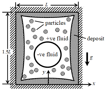
Figure 10 shows a cavity with a +ve fluid encapsulating a lighter -ve fluid bubble. The width and height of the cavity are respectively L and 1.5L. The +ve fluid contains initially a uniform suspension of particles. These particles deposit gradually on the four cavity walls forming a solid deposit layer. At the same time, the -ve fluid bubble rises under the effect of gravity. The deposit layer grows with time and it affects the motion of the bubble in a fully coupled manner. For this problem, the characteristic length and velocity are set to L and $u_{o}=\sqrt{g L}$ respectively. The bubble is located at x*=0 and y*=0.5. As the problem is symmetric, solution for the right half domain is computed using the following initial conditions.
$\vec{u}^{*}=\overrightarrow{0} \quad C^{*}=\left\{\begin{array}{ll}C_{o}^{*} & , \text { in }+\text { ve fluid } \\ 0 & \text { ,in }-\text { ve fluid }\end{array}\right.$ for $0 \leq x^{*} \leq 0.5$ and $0 \leq y^{*} \leq 1.5$ (18a)
At the left symmetry plane ( $\left.x^{*}=0,0 \leq y^{*} \leq 1.5\right) u^{*}=0, \frac{\partial v^{*}}{\partial x^{*}}=0 \quad \frac{\partial C^{*}}{\partial x^{*}}=0$ (18b)
Figure 10. Schematic of particle deposition in a cavity with a rising bubble
No slip and zero particle flux are enforced at all walls.
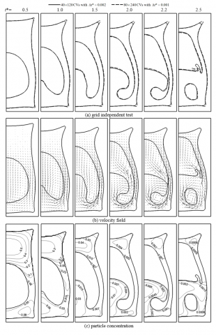
Again, the solution of a standard case will be first presented after which the effect of various dimensionless number is studied. For the standard case, $R / L=0.35, \rho_{-} / \rho_{+}=0.001, \mu_{-} / \mu_{+}=0.02$, Re=1980, Fr=1, We=9800, Pe=14.8, Da=10 and $C_{o}^{*}=0.5$. The solutions on two different meshes are shown in Figure 11a. the solution on the mesh of 40×120 CVs with Δt*=0.002 is considered mesh independent and therefore it will be used in all the consecutive computations. The corresponding velocity and particle concentration fields are plotted respectively in Figure 11b and 11c.
Initially, there are more particles in the upper region, as only the +ve fluid contains particles. The lower region is mainly occupied by the -ve fluid with smaller amount of +ve fluid. The particles deposit rapidly onto the walls with the deposit layer grows rapidly up to t*=1 after which it slows down. The maximum particle concentration drops from an initial value of C*=0.5 to C*=0.04 at t*=1.5, where practically the particles are almost depleted. Therefore, the growth of the deposit layer after t*=1.5 is minute and could no longer be visually distinguished easily. Overall, a much thicker deposit layer forms in the upper region. Simultaneously occurring together with deposition, the bubble rises, gravitationally driven, with two pairs of circulatory flow structure formed leading to its eventual break-up. Break-up of the bubble occurs very rapidly right after t*=2.2. A mesh with finer temporal and spatial resolution is needed to capture accurately the break-up process and hence the difference of the fluid-fluid interface seen at t*=2.5 in Figure 11a. Upon breaking up, two daughter bubbles form with one much smaller then the other. It should be mentioned that the effect of mesh resolution on the fluid-deposit front is minimum as would be reasonably expected given that most particles have already deposited much earlier prior to the break-up process.
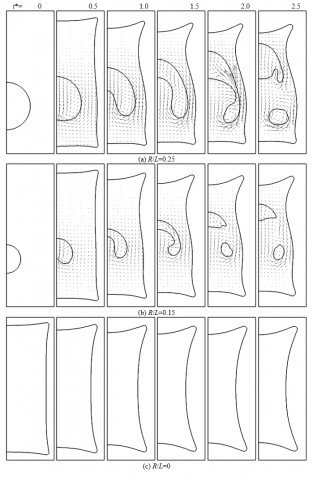
Shown in Figure 12 is the case with the bubble size reduces to R/L=0.25, 0.15 and 0. As the bubble size decreases, the region covered by the +ve fluid (containing particles) increases. Therefore, the total amount of particles available in the lower region increases with smaller bubble size. As such a generally thicker deposit layer is found in the lower region. The case of R/L=0 corresponds to the situation where there is no bubble. As the region now contains only the +ve fluid, no gravitational driven motion occurs. Diffusion is the only transport mechanism driving the particles to the front for deposition. The problem then becomes also symmetric at the plane of y*=0.75, leading to a symmetric deposit profile.
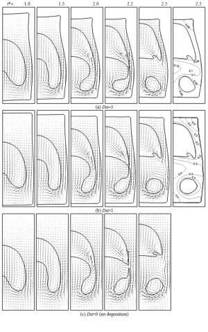
The effect of Da is now investigated by reducing Da from 10 of the standard case to Da=3, 1 and 0, i.e., increasingly reaction-controlled leading to a slower deposition process. The solutions are plotted in Fig. 13. The particle concentration at t*=2.5 for these cases is also given. For the case of Da=3, almost all particles are deposited at the end of the simulation at t*=2.5, inferred from the low particle concentration. However, the deposit profile in particular in the upper right region is markedly different from that of Da=10 in Figure 11. Generally the deposit thickness becomes more uniform in the upper right region. and the sharp creviced feature is no longer presence. Upon reducing to Da=1, the deposition process becomes even more slowly. In the upper right region, particle concentration is still high as C*=0.5 at t*=2.5. Instead of deposited, a lot of particles are still suspended in the +ve fluid. It takes time for particles to be deposited even if present right at the fluid-deposit front. Therefore, the deposition process is still in progress at t*=2.5. Finally, the case of Da=0 corresponds to the situation with no deposition. As can be easily noticed, the presence of the deposit layer intimately affect the motion and shape of the rising bubble. Without deposition, break-up occurs slightly earlier, i.e., prior to t*=2.2.
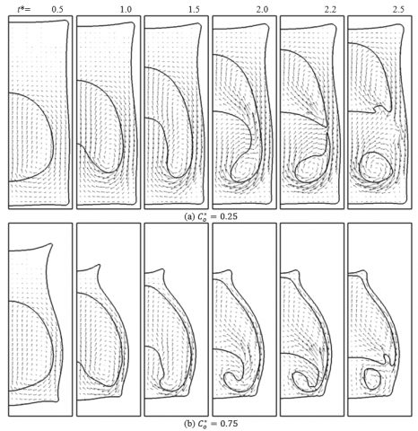
The initial concentration $C_{o}^{*}$ has a strong effect on the deposit thickness and eventually on the rising bubble. The solutions for the case with a smaller ( $C_{o}^{*}=0.25$ ) and larger ( $C_{o}^{*}=0.75$) initial concentration in comparison with the standard ( $C_{o}^{*}=0.5$ ) case are shown in Figure 14. For the case of $C_{o}^{*}=0.25$, the deposit layer remains thin even with all the particles deposited. It effects on the motion and shape of the rising bubble is small, see for example comparison of Figure 13c (no deposition) and Figure 14a at t*=2.5. The case of $C_{o}^{*}=0.75$ is more interesting. The deposit layer is thick particularly in the upper region effectively confining the bubble. Therefore, as the bubble rises, it has to deform in such a way to conform to the shape of the deposit layer. There is a +ve fluid layer between the -ve fluid bubble and the deposit. This +ve fluid layer becomes thinner as it is gradually squeezed by the rising bubble. Upon break-up a much smaller daughter bubble is formed given the more intricate dynamics of the interface.
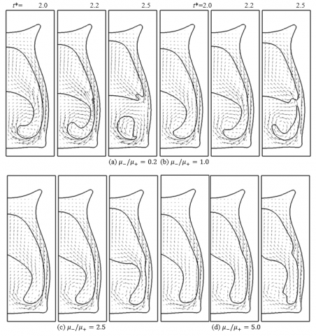
The effect of viscosity ratio is now considered. The viscosity ratio is increased from the standard case of $\mu_{-} / \mu_{+}=0.02$ to 0.2, 1.0, 2.5 and 5.0 as shown in Figure 15. Only solutions at t*=2.0, 2.2 and 2.5 are plotted. At least for the cases studied, the effect on the growth of the deposit layer is not significant given that the deposit formed earlier. A larger value is however expected if Da is lower, say 5.0. As $\mu_{-} / \mu_{+}$ is increased, the -ve fluid would have increasingly larger viscosity relative to that of the +ve fluid. The bubble becomes more difficult to deform and therefore break up. For $\mu_{-} / \mu_{+}=2.5$ and 5.0, no break up of the bubble occurs up to t*=2.5.
Figure 11. Solution for the standard case of a bubble rising in a cavity with deposition
Figure 12. Effect of R/L
Figure 13. Effect of Da
Figure 14. Effect of $C_{o}^{*}$
Figure 15. Effect of $\mu_{-} / \mu_{+}$
A numerical procedure to predict particle deposition in a two-fluid flow environment is presented in this article. For this type of problems, the velocity, pressure, particle concentration fields are strongly coupled altogether and with the evolving fluid-fluid interface and fluid-deposit front as well. Both interface and front are captured via the level-set method. At the fluid-deposit front, particles are assumed to deposit as a first order deposition reaction. The governing conservation equations are solved by employing a finite volume method. The procedure is verified against two limiting cases, i.e. fluid-fluid flow problem (rising bubble in a partially-filled container) and fluid flow with deposition problem (single-fluid flow in a channel with particle deposition). Then, applications of the procedure are demonstrated for particle deposition in a stratified two-fluid flow and in a cavity with a rising bubble. Via these demonstration cases, the effect of some of the dimensionless governing parameters is briefly investigated. Future work of interest includes that involving multi-species where there are more than one species of particles depositing simultaneously.
|
C |
particle concentration, kg/m3 |
|
Co |
initial particle concentration, kg/m3 |
|
d |
normal distance from interface, m |
|
D |
diffusion coefficient, m2/s |
|
Da |
Damkohler number |
|
Fr |
Froude number |
|
g |
gravitational acceleration, m/s2 |
|
h |
thickness of fluid layer, m |
|
H |
smoothed Heaviside function |
|
k |
deposition reaction rate, m/s |
|
L |
characteristic length, m |
|
$\hat{n}$ |
unit normal vector |
|
p |
Pressure, Pa |
|
Pe |
Peclet number |
|
$\vec{q}$ |
deposition flux, kg/m2s |
|
R |
radius of bubble, m |
|
Re |
Reynolds number |
|
t |
time, s |
|
u |
velocity component in x-direction, m/s |
|
uo |
characteristic velocity, m/s |
|
$\vec{u}$ |
velocity vector, m/s |
|
v |
velocity component in y-direction, m/s |
|
We |
Weber number |
|
Greek symbols |
|
|
δ |
smoothed Dirac delta function |
|
φ |
level-set function, m |
|
μ |
Viscosity, Pa.s |
|
ρ |
Density, kg/m3 |
|
σ |
surface tension, N/m |
|
Subscripts |
|
|
d |
fluid-deposit interface, or deposit |
|
f |
fluid-fluid interface |
|
+ |
+ve fluid |
|
- |
-ve fluid |
|
Superscript |
|
|
* |
dimensionless quantities |
[1] Alnaimat, F., Ziauddin, M. (2020). Wax deposition and prediction in petroleum pipelines. Journal of Petroleum Science and Engineering, 184: 106385. https://doi.org/10.1016/j.petrol.2019.106385
[2] Balakin, B.V., Lo, S., Kosinski, P., Hoffmann, A.C. (2016). Modelling agglomeration and deposition of gas hydrates in industrial pipelines with combined CFD-PBM technique. Chemical Engineering Science, 153: 45-57. http://dx.doi.org/10.1016/j.ces.2016.07.010
[3] Guan, Q., Goharzadeh, A., Chai, J.C., Vargas, F.M., Biswal, S.L., Chapman, W.G., Zhang, M., Yap, Y.F. (2018). An integrated model for asphaltene deposition in wellbores/pipelines above bubble pressures. Journal of Petroleum Science and Engineering, 169: 353-373. https://doi.org/10.1016/j.petrol.2018.05.042
[4] Li, W., Li, H.X., Li, G.Q., Yao, S.C. (2013). Numerical and experimental analysis of composite fouling in corrugated plate heat exchangers. International Journal of Heat and Mass Transfer, 63: 351-360. https://doi.org/10.1016/j.ijheatmasstransfer.2013.03.073
[5] Mavridou, S.G., Bouris, D.G. (2012). Numerical evaluation of a heat exchanger with inline tubes of different size for reduced fouling rates. International Journal of Heat and Mass Transfer, 55: 5185-5195. https://doi.org/10.1016/j.ijheatmasstransfer.2012.05.020
[6] Xu, Z, Han, Z., Sun, A., Yu, X. (2019). Numerical study of particulate fouling characteristics in a rectangular heat exchange channel. Applied Thermal Engineering, 154: 657-667. https://doi.org/10.1016/j.applthermaleng.2019.03.142
[7] Sethian, J.A., Shan, Y. (2008). Solving partial differential equations on irregular domains with moving interfaces, with applications to superconformal electrodeposition in semiconductor manufacturing. Journal of Computational Physics, 227: 6411-6447. https://doi.org/10.1016/j.jcp.2008.03.001
[8] Barua, H., Povitsky, A. (2020). Numerical model of carbon chemical vapor deposition at internal surfaces. Vacuum, 175: 109234. https://doi.org/10.1016/j.vacuum.2020.109234
[9] Adalsteinsson, D., Sethian, J.A. (1995). A level set approach to a unified model for etching, deposition, and lithography I: Algorithms and two-dimensional simulations. Journal of Computational Physics, 120: 128-144. https://doi.org/10.1006/jcph.1995.1153
[10] Sun, Z., Guo, W., Li. L. (2020). Numerical modelling of heat transfer, mass transport and microstructure formation in a high deposition rate laser directed energy deposition process. Additive Manufacturing, 33: 101175. https://doi.org/10.1016/j.addma.2020.101175
[11] Caraghiaur, D., Anglart, H. (2013). Drop deposition in annular two-phase flow calculated with Lagrangian Particle Tracking. Nuclear Engineering and Design, 265: 856-866. https://doi.org/10.1016/j.nucengdes.2013.06.026
[12] Alam, S. (2016). Mathematical modelling for the effects of thermophoresis and heat generation /absorption on MHD convective flow along an inclined stretching sheet in the presence of dufour-soret effects. Mathematical Modelling of Engineering Problems, 3: 119-128. https://doi.org/10.18280/ mmep.030302
[13] Fasogbon, S.K., Oyelami, F.H., Adetimirin, E.O., Ige, E.O. (2019). On Blasius Plate Solution of Particle Dispersion and Deposition in Human Respiratory Track. Mathematical Modelling of Engineering Problems, 3: 428-432. https://doi.org/10.18280/mmep. 060314
[14] Swain, K. (2019). A study on MHD nanofluid flow and heat transfer with convective surface temperature and concentration. Modelling, Measurement and Control B, 88: 73-78. https://doi.org/10.18280/mmc_b.882-405
[15] Pourhashem, H., Owen, M.P., Castro, N.D., Rostami, A.A. (2020). Eulerian modeling of aerosol transport and deposition in respiratory tract under thermodynamic equilibrium condition. Journal of Aerosol Science, 141: 105501. https://doi.org/10.1016/j.jaerosci.2019.105501
[16] Zhang, Z., Chen Q. (2007). Comparison of the Eulerian and Lagrangian methods for predicting particle transport in enclosed spaces. Atmospheric Environment, 41: 5236-5248. https://doi.org/10.1016/j.atmosenv.2006.05.086
[17] Hryb, D., Cardozo, M., Ferro, S., Goldschmit, M. (2009). Particle transport in turbulent flow using both Lagrangian and Eulerian formulations. International Communications in Heat and Mass Transfer, 36: 451-457. https://doi.org/10.1016/j.icheatmasstransfer.2009.01.017
[18] Wieland, C., Kreutzkam, B., Balan, G., Spliethoff, H. (2012). Evaluation, comparison and validation of deposition criteria for numerical simulation of slagging. Applied Energy, 93: 184-192. https://doi.org/10.1016/j.apenergy.2011.12.081
[19] Guha, A. (1997). A unified Eulerian theory of turbulent deposition to smooth and rough surfaces. Journal of Aerosol Science, 28: 1517-1537. https://doi.org/10.1016/S0021-8502(97)00028-1
[20] Abdolzadeh, M., Mehrabian, M.A., Goharrizi, A.S. (2011). Numerical study to predict the particle deposition under the influence of operating forces on a tilted surface in the turbulent flow. Advanced Powder Technology, 22: 405-415. https://doi.org/10.1016/ j.apt.2010.06.005
[21] Suh, S.M., Zachariah, M.R., Girshicka, S.L. (2002). Numerical modeling of silicon oxide particle formation and transport in a one-dimensional low-pressure chemical vapor deposition reactor. Aerosol Science, 33: 943-959. https://doi.org/10.1016/S0021-8502(02)00047-2
[22] Bar, E., Lorenz, J., Ryssel, H. (2002). Simulation of the influence of via sidewall tapering on step coverage of sputter-deposited barrier layers. Microelectronic Engineering, 64: 321-328. https://doi.org/10.1016/S0167-9317(02)00805-5
[23] Vargas, F.M., Creek, J.L., Chapman, W.G. (2010). On the development of an asphaltene deposition simulator. Energy & Fuels, 24: 2294-2299. https://doi.org/10.1021/ef900951n
[24] Ge, Q., Yap, Y.F., Vargas, F.M., Zhang, M., Chai, J.C. (2012). A total concentration method for multi-species particle deposition process. ISTP23-116, 23rd International Symposium on Transport Phenomena, Nov 19-22, Auckland, New Zealand.
[25] Yap, Y.F., Vargas, F.M., Chai, J.C. (2013). A level-set method for multi-species particle deposition. Proc. of the ASME 2013 Summer Heat Transfer Conference, Jul 14-19, Minneapolis, MN, USA.
[26] Heitzinger, C., Selberherr, S. (2002). On the topography simulation of memory cell trenches for semiconductor manufacturing deposition processes using the level set method. Proceedings of 16th European Simulation Multiconference: Modelling and Simulation 2002 (ESM 2002), Jun. 3-5, Darmstadt, Germany, 653-660.
[27] Hughes, M., Strussevitch, N., Bailey, C., McManus, K., Kaufmann, J., Flynn, D., Desmulliez, M.P.Y. (2010). Numerical algorithms for modelling electrodeposition: Tracking the deposition front under forced convection from megasonic agitation. International Journal for Numerical Methods in Fluids, 64: 237-268. https://doi.org/10.1002/fld.2140
[28] Lawal, K.A., Vesovic, V., Boek, E.S. (2011). Modeling permeability impairment in porous media due to asphaltene deposition under dynamic conditions. Energy & Fuels, 25: 5647-5659. https://doi.org/10.1021/ef200764t
[29] Zhu, Z., Sand, K.W., Teevens, P.J. (2010). A numerical study of under-deposit pitting corrosion in sour petroleum pipelines. Northern Area Western Conference, Feb. 15-18, Calgary, Alberta.
[30] Chen, Z., Liu, S. (2010). Simulation of copper electroplating fill process of through silicon via. Packaging Technology, 3: 433-437. https://doi.org/10.1109/ICEPT.2010.5583828
[31] Helmsen, J.J. (1996). Volume of fluids methods applied to etching and deposition. American Physical Society, Gaseous Electronics Conference, Oct. 21-24.
[32] Yap, Y.F., Vargas, F.M., Chai, J.C. (2013). A level-set method for convective-diffusive particle deposition. Applied Mathematical Modelling, 37: 5245-5259. https://doi.org/10.1016/j.apm.2012.10.039
[33] Banki, R., Hoteit, H., Firoozabadi, A. (2008). Mathematical formulation and numerical modeling of wax deposition in pipelines from enthalpy–porosity approach and irreversible thermodynamics. International Journal of Heat and Mass Transfer, 51: 3387-3398. https://doi.org/10.1016/j.ijheatmasstransfer.2007.11.012
[34] Ge., Q., Yap, Y.F., Vargas, F.M., Zhang, M., Chai, J.C. (2012). A total concentration method for modeling of deposition. Numerical Heat Transfer, Part B: Fundamentals, 61: 311-328. https://doi.org/10.1080/10407790.2012.670582
[35] Yan, X., Chen, G. (2021). An approximation approach for the simulation of vapor-liquid phase change by the volume-of-fluid method, International Journal of Multiphase Flow, 136: 103359. https://doi.org/10.1016/j.ijmultiphaseflow.2020.103359
[36] Li, Q., Dong, F., Li, L.K.B. (2020). An interface-sharpening method with adaptive mesh refinement for volume-of-fluid simulations of two-phase compressible flows. Computers & Fluids, 210: 104648. https://doi.org/10.1016/j.compfluid.2020.104648
[37] Xie, Z., Stoesser, T. (2020). A three-dimensional Cartesian cut-cell/volume-of-fluid method for two-phase flows with moving bodies. Journal of Computational Physics, 416: 109536. https://doi.org/10.1016/j.jcp.2020.109536
[38] Lyras, K.G., Hanson, B., Fairweather, M., Heggs, P.J. (2020). A coupled level set and volume of fluid method with a re-initialisation step suitable for unstructured meshes. Journal of Computational Physics, 407: 109224. https://doi.org/10.1016/j.jcp.2019.109224
[39] Huang, Z., Senra, M., Kapoor, R., Fogler, H.S. (2011). Wax deposition modeling of oil/water stratified channel flow. AIChE Journal, 57: 841-85. https://doi.org/10.1002/aic.12307
[40] Ramirez-Jaramillo, E., Lira-Galeana, C., Manero, O. (2006). Modeling asphaltene deposition in production pipelines. Energy & Fuels, 20: 1184-1196. https://doi.org/10.1021/ef050262s
[41] Van Parys, H., Nierhaus, T., Dehaeck, S., van Beeck, J., Deconinck, J., Hubin, A. (2008). Numerical simulation of an electro-deposition reaction under two-phase flow conditions. 213th ECS Meeting, Abstract #882, May 18-22, Phoenix, Arizona.
[42] Osher, S., Sethian, J.A., (1988). Fronts propagating with curvature-dependent speed: Algorithms based on Hamilton-Jacobi formulations. Journal of Computational Physics, 79: 12-49. https://doi.org/10.1016/0021-9991(88)90002-2
[43] Sussman, M., Smereka, P., Osher, S. (1994). A level set approach for computing solution to incompressible two-phase flow. Journal of Computational Physics, 114: 146-159. https://doi.org/10.1006/jcph.1994.1155
[44] Peng, D., Merriman, B., Osher, S., Zhao, H., Kang, M. (1999). A PDE-based fast local level-set method. Journal of Computational Physics, 155: 410-438. https://doi.org/10.1006/jcph.1999.6345
[45] Yap, Y.F., Chai, J.C., Wong, T.N., Toh, K.C., Zhang, H.Y. (2006). A global mass correction scheme for the level-set method. Numerical Heat Transfer B: Fundamentals 50-5: 455-472. https://doi.org/10.1080/10407790600646958
[46] Yap, Y.F., Chai, J.C., Toh, K.C., Wong, T.N., Lam, Y.C. (2005). Numerical modeling of unidirectional stratified flow with and without phase change. International Journal of Heat and Mass Transfer, 48: 477-486. https://doi.org/10.1016/j.ijheatmasstransfer.2004.09.017
[47] Chen, S., Merriman, B., Osher, S., Smereka, P. (1995). A simple level set method for solving Stefan problems. Journal of Computational Physics, 135: 8-29. https://doi.org/10.1006/jcph.1997.5721
[48] Brackbill, J.U., Kothe, D.B., Zemach, C. (1992). A continuum method for modelling surface tension. Journal of Computational Physics, 100: 335-354. https://doi.org/10.1016/0021-9991(92)90240-Y
[49] Patankar, S.V. (1980). Numerical Heat Transfer and Fluid Flow. Hemisphere Publisher.
[50] Versteeg, H.K., Malalasekera, W. (2007). An Introduction to Computational Fluid Dynamics: The Finite Volume Method, 2nd ed. Prentice Education Limited.
[51] Roe, P.L. (1986). Characteristic-based schemes for the Euler equations. Annual Review of Fluid Mechanics, 18: 337-365. https://doi.org/10.1146/annurev.fl.18.010186.002005
[52] Jiang, G.S., Peng, D. (2000). Weighted ENO schemes for Hamilton-Jacobi equations. SIAM Journal on Scientific Computing, 21: 2126-2143. https://doi.org/10.1137/S106482759732455X
[53] Shu, C.W., Osher, S. (1988). Efficient implementation of essentially non-oscillatory shock capturing schemes. Journal of Computational Physics, 77: 439-471. https://doi.org/10.1016/0021-9991(88)90177-5
[54] Sheu, T.W.H., Yu, C.H., Chiu, P.H. (2009). Development of a dispersively accurate conservative level set scheme for capturing interface in two-phase flows. Journal of Computational Physics, 228: 661-686. https://doi.org/10.1016/j.jcp.2008.09.032
[55] Zhao, Y., Tan, H.H., Zhang, B. (2002). A high-resolution characteristics-based implicit dual time-stepping VOF method for free surface flow simulation on unstructured grids. Journal of Computational Physics, 183: 233-273. https://doi.org/10.1006/jcph. 2002.7196