Risk Assessment of Smart Community Heating Reconstruction Project Based on Artificial Neural Network

Smart community heating reconstruction has just started in China. There are not many technologies or investment cases for reference. Besides, any community heating reconstruction project faces lots of uncertainties, which arise from the geographic location, layout, and building features of the communities. Similarly, uncertain factors abound throughout project construction. To a certain extent, the distribution law and change mechanism of these factors are stochastic and fuzzy. The stochasticity and fuzziness must be fully considered to assess the risks of smart community heating reconstruction projects.

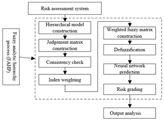
Figure 1 shows the risk assessment model for smart community heating reconstruction projects. To improve the accuracy of project decision-making, this paper firstly constructs a fuzzy set that is randomly projected by the law of large numbers, and then evaluates the smart community heating reconstruction risks based on fuzzy mathematics and set-valued statistics.

1.png

Figure 1. Risk assessment system for smart community heating reconstruction projects

This paper constructs a hierarchical risk assessment system for smart community heating reconstruction projects, which covers four aspects: market aspect, technical design, project investment, and heating reliability.

Layer 1 (goal layer):

HRR={risk assessment of smart community heating reconstruction};

Layer 2 (criteria layer):

HRR={HRR₁, HRR₂, HRR₃, HRR₄}={market aspect, technical design, project investment, heating reliability};

Layer 3 (alternative layer):

HRR₁={HRR₁₁, HRR₁₂, HRR₁₃, HRR₁₄, HRR₁₅, HRR₁₆}={real-time electricity price, real-time heating price, heat source heating cost, grid power supply cost, risk of public opinion, operating risk of reconstructed system};

HRR₂={HRR₂₁, HRR₂₂, HRR₂₃, HRR₂₄, HRR₂₅, HRR₂₆, HRR₂₇, HRR₂₈, HRR₂₉}={rationality of technical solution, completeness of equipment, professionalism of personnel, reliability of installation and commissioning, controllability of project construction and coordination, operating stability of original and reconstructed system, reliability of power supply, safety of relay protection, protection of power quality};

HRR₃={HRR₃₁, HRR₃₂, HRR₃₃, HRR₃₄, HRR₃₅, HRR₃₆, HRR₃₇, HRR₃₈}={investment fund, construction cycle, operating investment cost, additional investment cost, energy efficiency evaluation, profitability, development capacity, operating capacity};

HRR₄={HRR₄₁, HRR₄₂, HRR₄₃, HRR₄₄, HRR₄₅, HRR₄₆}={operating reliability, equipment aging, equipment damage, pipeline aging, climate and geographical factors, generator power}.

Out of the 28 secondary indices, the indices that significantly affect the risk assessment of smart community heating reconstruction and change greatly over time were taken as risk factors. Let v_i be the i-th risk factor. Then, the set of risk factors can be expressed as:

$V=\left\{ {{v}_{1}},{{v}_{2}},...,{{v}_{m}} \right\}$      (1)

This paper defines the degree of variation of a risk assessment index with influencing factors as the sensitivity of its risk factor. The sensitivity ξ_i of an index to a risk factor v_i can be expressed as:

${{\xi }_{i}}=\left| \frac{\frac{dHHR}{HHR}}{\frac{d{{v}_{i}}}{{{v}_{i}}}} \right|=\left| \frac{dHHR}{d{{v}_{i}}}\frac{{{v}_{i}}}{HHR} \right|\text{  }\left( i=1,2,...,n \right)$       (2)

Similarly, the sensitivity ξ_i^(l) of index HHR to the i-th risk factor v_i in period l can be expressed as:

$\xi _{_{i}}^{\left( l \right)}=\left| \frac{\frac{dHH{{R}^{\left( l \right)}}}{HH{{R}^{\left( l \right)}}}}{\frac{dv_{_{i}}^{\left( l \right)}}{v_{_{i}}^{\left( l \right)}}} \right|=\left| \frac{dHH{{R}^{\left( l \right)}}}{dv_{_{i}}^{\left( l \right)}}\frac{v_{_{i}}^{\left( l \right)}}{HH{{R}^{\left( l \right)}}} \right|\text{  }\left( i=1,2,...,n;l=1,2,...,m \right)$       (3)

The value of ξ_i can be calculated by:

${{\xi }_{i}}=\frac{1}{m}\sum\limits_{l=1}^{m}{\xi _{_{i}}^{\left( l \right)}}\text{ }\left( i=1,2,...,n \right)$       (4)

The normalized value ξ_i^* of ξ_i can serve as the weight coefficient of risk factors:

$\xi _{i}^{*}=\frac{{{\xi }_{i}}}{\sum\limits_{i=1}^{n}{{{\xi }_{i}}}}\text{ }\left( i=1,2,...,n \right)$      (5)

Table 1 lists the sensitivities of the four primary indices.

Table 1. Sensitives of primary indices

Lacking investment experience, the decision-makers want to make objective decisions about whether or not to invest in smart community heating reconstruction through quantitative analysis of the reconstruction project. If expert method is adopted to evaluate the risk attributes of the project, the evaluation will be greatly affected by the expertise and preference of the experts. The set-valued statistics provides an effective way to ease the subjective interference. This approach views a fuzzy risk factor as a random variable that can be characterized with an interval. By set-valued statistics, the risk factors can be counted in a fuzzy manner, while making objective decisions and fuzzy judgements. The interval of the value of a risk factor estimated by the i-th expert can be defined as:

${{\sigma }_{i}}=\left[ {{a}_{i,}}a_{i}^{'} \right]\text{   }\left( j=1,2,...,k \right)$      (14)

According to the principle of set-valued statistics, the assessment index of the risk factor can be described by a convex membership function Ã:

$\tilde{A}=g\left( a \right)=\frac{1}{k}\left( \sum\limits_{i=1}^{k}{\Phi _{{{\sigma }_{i}}}^{\left( a \right)}} \right)$      (15)

where, Φ_σi^(a) is a binary function reflecting whether a falls in the interval of estimated value:

$\Phi _{_{{{\sigma }_{i}}}}^{\left( a \right)}=\left\{ \begin{align}  & 1\text{   }a\in \left[ {{a}_{i,}}a_{j}^{'} \right]={{\delta }_{i}} \\ & 0\text{   }a\notin \left[ {{a}_{i,}}a_{j}^{'} \right]={{\delta }_{i}} \\\end{align} \right.$     (16)

Combining formulas (15) and (16):

$\tilde{A}=g\left( a \right)=\left\{ \begin{align}  & {{l}_{1}}\text{   }a\in \left[ {{e}_{1}},{{e}_{2}} \right) \\ & {{l}_{2}}\text{   }a\in \left[ {{e}_{2}},{{e}_{3}} \right) \\ & \vdots \text{       }\vdots  \\ & {{l}_{m}}\text{   }a\in \left[ {{e}_{m}},{{e}_{m+1}} \right] \\\end{align} \right.$      (17)

à can be normalized as:

$\int_{{{e}_{1}}}^{{{e}_{n+1}}}{\overset{\tilde{\ }}{\mathop{A}}\,{{r}_{a}}}=\sum\limits_{i=1}^{m}{{{l}_{i}}}\left( {{e}_{i+1}}-{{e}_{i}} \right)=p$      (18)

Then, the normalized convex membership function of à can be expressed as:

$\dot{A}=\dot{g}\left( x \right)=\left\{ \begin{align}  & \frac{{{l}_{1}}}{p}\text{   }a\in \left[ {{e}_{1}},{{e}_{2}} \right) \\ & \frac{{{l}_{2}}}{p}\text{   }a\in \left[ {{e}_{1}},{{e}_{2}} \right) \\ & \vdots \text{       }\vdots  \\ & \frac{{{l}_{m}}}{p}\text{   }a\in \left[ {{e}_{m}},{{e}_{m+1}} \right] \\\end{align} \right.$     (19)

The normalized convex membership function is constrained by:

$\int_{{{e}_{1}}}^{{{e}_{n+1}}}{\dot{A}{{r}_{a}}}=1$      (20)

The expectation DV(A) of the assessment index of the risk factor can be given by:

$DV\left( A \right)=\int_{{{e}_{1}}}^{{{e}_{m+1}}}{\overset{\hat{\ }}{\mathop{A}}\,ada}=\frac{1}{2p}\sum\limits_{i=1}^{m}{{{l}_{i}}}=\left( e_{_{i+1}}^{2}-e_{_{i}}^{2} \right)$      (21)

The corresponding variance VC(A) can be described by:

$\begin{align}  & VC\left( A \right)=\int_{{{e}_{1}}}^{{{e}_{m+1}}}{\overset{\hat{\ }}{\mathop{A}}\,{{\left[ a-DV\left( A \right) \right]}^{2}}r\left( a \right)}= \\ & \frac{1}{3p}\sum\limits_{i=1}^{m}{{{l}_{i}}}\left\{ {{\left[ e_{_{i+1}}^{2}-DV\left( A \right) \right]}^{3}}-{{\left[ {{e}_{i}}-DV\left( A \right) \right]}^{3}} \right\} \\\end{align}$      (22)

The standard deviation BD(A) can be calculated by:

$BD\left( A \right)=\sqrt{VC\left( A \right)}$      (23)

Then, the interval of the maximum possible value of the assessment index for the risk factor can be defined as:

$VC=\left[ DV\left( A \right)-BD\left( A \right),DV\left( A \right)+BD\left( A \right) \right]$      (24)

Suppose the interval satisfies:

${{\sigma }_{i}}\cap VC=\left[ {{r}_{i}},r_{_{i}}^{'} \right]\text{    }\left( i=1,2,...,k \right)$     (25)

The expected estimation fuzziness w_ij of the i-th expert for the j-th risk factor can be calculated by:

${{w}_{ij}}=r_{_{i}}^{'}-{{r}_{i}}$     (26)

The expected estimation fuzziness w^'_j of all experts for the j-th risk factor can be calculated by:

$w_{j}^{'}=\sum\limits_{i=1}^{k}{{{w}_{ij}}}$      (27)

If the experts are uncertain about the estimated interval, w_ij=0. The assessment reliability η_ij of the i-th expert for the j-th risk factor can be calculated by:

${{\eta }_{ij}}=\frac{{{w}_{ij}}}{2BD\left( A \right)}\text{    }\left( i=1,2,...,k \right)$      (28)

The comprehensive assessment reliability S of all experts for the j-th risk factor can be calculated by:

$S=\frac{w_{j}^{'}}{2BD\left( A \right)}$      (29)

The normalized result θ_ij of η_ij can be expressed as:

${{\theta }_{ij}}=\frac{{{s}_{ij}}}{\sum\limits_{i=1}^{k}{{{s}_{ij}}}}$      (30)

θ_ij satisfies Σ^k_i=1θ_ij=1. Formula (30) shows that the θ_ij value increases with the level of the i-th expert. Smart community heating reconstruction involves many risk factors. Therefore, the assessment of the reconstruction risks is a multi-factor comprehensive assessment. If multiple experts are invited to assess the risks of the heating reconstruction in the same smart community, then the assessment reliability W_i of the i-th expert for all risk factors can be quantified by:

${{W}_{i}}=\frac{1}{n}\sum\limits_{j=1}^{n}{{{\theta }_{ij}}}\text{    }\left( i=1,2,...,k \right)$      (31)

W_i characterizes the reliability of the subjective, empirical judgement of each expert. It can be taken as the weight coefficients of secondary indices. Since W={W₁, W₂, …, W_k} satisfies Σ^k_i=1W_i=1, the risk assessment model for smart community heating reconstruction can be given by:

$S=W\cdot F=\left( {{f}_{1}},{{f}_{2}},...,{{f}_{m}} \right)$      (32)

where, f_j can be calculated by:

${{f}_{j}}=\sum\limits_{i=1}^{k}{{{W}_{i}}}{{f}_{ij}}\left( j=1,2,...,m \right)$      (33)

By the principle of maximum membership, f_j= max{f₁, f₂, …, f_m}. The risk grade of the target smart community heating reconstruction project is denoted as grade u_j.

This section firstly analyzes the internal correlations between the estimated intervals of the risk assessment indices for smart community heating reconstruction. Table 2 sorts the secondary indices by the cumulative variance explained (CVE).

Table 2 shows that the CVE of secondary indices contained eight eigenvalues that are greater than 1: 4.427, 4.128, 2.315, 2.159, 1.721, 1.434, 1.190, and 1.021. The CVE of the eight secondary indices reached 82.489%, suggesting that these indices can reflect most risk features of Chinese old community heating reconstruction projects. Similarly, eight key risk factors could be extracted from the scree plot of the risk assessment system (Figure 4).

Table 2. CVE of each risk assessment index

4.png

Figure 4. Scree plot of the risk assessment system

5.png

Figure 5. Iterative effect of the ASFA

6.png

Figure 6. Curve of training error

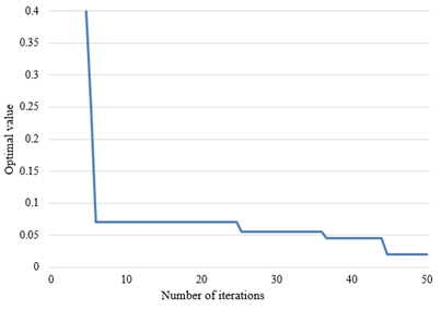
In addition, an experiment was designed to verify the effectiveness of the risk assessment model based on AFSA-optimized BPNN for smart community heating reconstruction projects. Firstly, the various parameters of the model were initialized, including learning rate, target training error, maximum number of iterations, incentive functions, learning function, training function, etc. The AFSA can update the initial connection weights and thresholds of the neural network. The termination condition of the AFSA is that the error falls below the target error, or the number of iterations reaches the maximum. Figure 5 shows the iterative effect of the ASFA.

As shown in Figure 5, BPNN was optimized ideally by the AFSA, which has a certain global convergence ability. Based on the AFSA-optimized BPNN, the proposed risk assessment model is highly feasible and researchable for smart community heating reconstruction. Next, 50 training samples were imported to the model for training. During the training, the model loss error was recorded as a curve, that is, the mean squared error (MSE) curve in Figure 6.

As shown in Figure 6, the AFSA-optimized BPNN basically tended to be stable after six iterations. The error fluctuated around 0.01. Hence, the optimization effectively overcomes the proneness of traditional BPNN to local optimum trap. After that, the risk grading effect of the improved BPNN was evaluated with 10 test samples. Table 3 provides the input layer data of the 10 test samples.

After that, the input layer data of the 10 test samples were imported to the AFSA-optimized BPNN for verification. The risk grading results of community heating reconstruction of the ten test samples are presented in Table 4.

As shown in Table 4, the accuracy of the risk grading on the ten test samples was as high as 90%. Only 1 item was misjudged, whose actual risk grade is good. The risk gradings of all the other items (whose actual risk grade is healthy, general, light risk, and heavy risk) were 100% correct. Therefore, the poorer the actual risk grade, the better the judgement by the proposed model. The results confirm that our model accurately judge the risk grades of community heating reconstruction in the 10 test samples, and could be applied to assess the risks of community heating reconstruction projects.

To verify the effectiveness of AFSA optimization for traditional BPNN, the original and improved models were tested on 15 samples. The risk assessment results of the original and improved models were summarized and compared in details. The judgement results (Figures 7 and 8) show that the improved model outputs more realistic risk grades than the original model. Table 5 compares the risk grades predicted by original and improved models.

As shown in Table 5, the improved model correctly identified 56.6% of the risk grades on the test samples. The only mistakes are about a sample of good risk and a sample of general risk. In this way, the judgement accuracy becomes much higher than that (1/2) of traditional BPNN. In practice, this paper provides a reference for the risk grading of smart community heating reconstruction in China through FCE and AFSA optimization. With the help of the model, investors and experts can evaluate the risk state of the specific community heating reconstruction project, and reasonably allocate their focus and funds to the project.

Table 3. Input layer data of the 10 test samples

Table 4. Risk grading results of community heating reconstruction

Table 5. Risk grades predicted by original and improved models

7.png

Figure 7. Risk grades estimated by traditional BPNN and the actual situation

8.png

Figure 8. Risk grading of the improved model vs. the actual risks