Mixed Convection in a Two-Sided and Four-Sided Lid-Driven Square Porous Cavity

2.1 Physical description

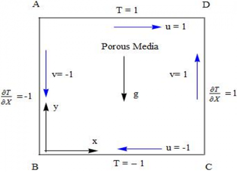
The physical model of a two-sided and four-sided lid-driven square cavity of unit size with heat transfer is illustrated in Figure 1. The cavity is filled with homogeneous, isotropic, saturated, sparsely packed porous material of high permeability K. The fluid's thermo-physical properties are presumed to be constant, except the density, which varies linearly with temperature as, $\rho=\rho_{0}\left[1-\beta\left(T_{h}-T_{c}\right)\right]$, where β is the thermal expansion coefficient, and the subscript 0 denotes the reference state. Natural convection occurs in the cavity due to temperature gradient, and forced convection occurs due to the motions of the lids. Thus, the combination of natural convection and forced convection results in a mixed convection problem.

In the two-sided porous cavity, the top and the bottom walls of the cavity move from left to right with velocity u = 1. The left and right walls of the porous cavity are maintained at cold (T =-1) and hot (T = 1) temperatures, respectively, while the top and the bottom walls of the cavity are adiabatic. In a four-sided cavity, the top and the bottom walls of the cavity move in opposite directions with velocity u = 1. The left and right walls of the cavity move with velocity v = 1 in the opposite directions. The top and the bottom walls of the porous cavity are maintained at hot (T = 1) and cold (T = -1) temperatures, respectively, while the left and right walls of the cavity are kept with heat flux $\partial T / \partial x=-1$ and $\partial T / \partial x=1$ respectively.

1a.png

(a) Two-sided lid-driven square porous cavity

1b.png

(b) Four-sided lid-driven square porous cavity

Figure 1. Flow configuration and coordinate system for two-sided and four-sided lid-driven square cavity in the porous media

2.2 Governing equations

The governing equations of mixed convection in a lid-driven square porous cavity based on Boussinesq approximations, using the stream function-vorticity $(\psi-\xi)$ formulation in the non-dimensional form [1] can be expressed as:

$\frac{1}{\varepsilon} \frac{\partial \xi}{\partial t}+\frac{1}{\varepsilon^{2}} u \frac{\partial \xi}{\partial x}+\frac{1}{\varepsilon^{2}} v \frac{\partial \xi}{\partial y}=\frac{G r}{2} \frac{\partial T}{\partial y}+\Lambda\left(\frac{\partial^{2} \xi}{\partial x^{2}}+\frac{\partial^{2} \xi}{\partial y^{2}}\right)-\frac{1}{D a} \xi$                       (1)

$S \frac{\partial T}{\partial t}+u \frac{\partial T}{\partial x}+v \frac{\partial T}{\partial y}=\frac{1}{P r}\left(\frac{\partial^{2} T}{\partial x^{2}}+\frac{\partial^{2} T}{\partial y^{2}}\right)$,            (2)

$\nabla^{2} \psi=-\xi$,            (3)

$u=\frac{\partial \psi}{\partial y}, v=-\frac{\partial \psi}{\partial x}$.                    (4)

where,

$\begin{align}  & \xi =\frac{\partial v}{\partial x}-\frac{\partial u}{\partial y},x=\frac{{{x}'}}{L},y=\frac{{{y}'}}{L},u=\frac{{{u}'}}{\alpha /L},v=\frac{{{v}'}}{\alpha /L},t=\frac{{{t}'}}{{{\alpha }^{2}}/L} \\  & \xi =\frac{\omega }{{{\alpha }^{2}}/L},\psi =\frac{{{\psi }'}}{L},T=\frac{\theta -{{\theta }_{0}}}{{{\theta }_{h}}-{{\theta }_{c}}},\theta =\frac{{{\theta }_{h}}+{{\theta }_{c}}}{2},{{\nabla }^{2}}=\frac{{{\partial }^{2}}}{\partial {{x}^{2}}}+\frac{{{\partial }^{2}}}{\partial {{y}^{2}}} \\ \end{align}$                     (5)

The non-dimensional parameters are Prandtl number, Darcy number, viscosity ratio and Grashof number, defined as follows:

$\operatorname{Pr}=\frac{v}{\alpha}, D a=\frac{K}{L^{2}}, \Lambda=\frac{\mu^{\prime}}{\mu}, G r=\frac{g \beta\left(\theta_{h}-\theta_{c}\right) L^{3}}{v^{2}}$.

The Darcy number is the ratio of permeability of the porous media to square of the length of the cavity. The medium’s permeability is defined as, $K=D_{p}^{2} \varepsilon^{2} / 144(1-\varepsilon)^{2}$, where D_p is the particle diameter and ε its porosity. The porosity in the porous media structure is an important indicator, which directly affects the movement characteristics of the fluid. So, its effect can be considered by varying the Darcy number.

The initial and the boundary conditions associated with the system (1) to (4) are:

Case 1: Two-sided lid-driven porous cavity

$t=0 ; u=v=T=\psi=\xi=0,0 \leq x, y \leq 1$,

$t>0 ; x=0: T=-1, \psi=\frac{\partial \psi}{\partial x}=0(i . e . v=0)$,

$x=1: T=1, \psi=\frac{\partial \psi}{\partial x}=0(i . e . v=0)$,

$y=0,1: \frac{\partial T}{\partial y}=0, \psi=0, \frac{\partial \psi}{\partial y}=1(i . e . u=1)$.

Case 2: Four-sided lid-driven porous cavity

$t=0 ; u=v=T=\psi=\xi=0, \quad 0 \leq x, y \leq 1$,

$t>0 ; x=0: \frac{\partial T}{\partial x}=-1, \psi=0, \frac{\partial \psi}{\partial x}=1(i . e, v=-1)$,

$x=1: \frac{\partial T}{\partial x}=1, \psi=0, \frac{\partial \psi}{\partial x}=-1(i . e . v=1)$,

$y=0: T=-1, \psi=0, \frac{\partial \psi}{\partial y}=-1(i . e . u=-1)$,

$y=1: T=1, \psi=0, \frac{\partial \psi}{\partial y}=1(i . e . u=1)$.

Heat transfer along the left and right walls of the cavity is also studied with the help of the average Nusselt number. The local and average Nusselt numbers along the left and right wall of the enclosure are defined as follows:

This section proves the stability and convergence of the considered problem using the Matrix method. We will adopt the following difference approximation formula for first-order partial derivatives [20]:

$D_{(+, x)}(\Delta x) \xi_{\mathrm{i}, \mathrm{j}}=\frac{\xi_{\mathrm{i}+1, \mathrm{j}}-\xi_{\mathrm{i}, \mathrm{j}}}{\Delta x}+O(\Delta x)$,

$D_{(-, x)}(\Delta x) \xi_{\mathrm{i}, \mathrm{j}}=\frac{\xi_{\mathrm{i}, \mathrm{j}}-\xi_{\mathrm{i}-1, \mathrm{j}}}{\Delta x}+O(\Delta x)$,

$D_{(0, x)}(\Delta x) \xi_{\mathrm{i}, \mathrm{j}}=\frac{\xi_{\mathrm{i}+1, \mathrm{j}}-\xi_{\mathrm{i}-1, \mathrm{j}}}{2 \Delta x}+O\left(\Delta x^{2}\right)$.

The second-order partial derivatives will be approximated by second-order central difference formula.

$D_{(0, x)}^{2}(\Delta x) \xi_{i, j}=\frac{\xi_{i+1, j}-2 \xi_{i, j}+\xi_{i-1, j}}{\Delta x^{2}}+O\left(\Delta x^{2}\right)$,

where, $\Delta x$ is the step length in x-direction. Similar formula will be adopted for $\mathrm{y}$ -direction. Let $\Delta t$ denotes the step length in time $(t)$ -direction. Further, we assume $A^{*}=$ $D_{0, x}^{2}, B^{*}=D_{0, y}^{2}, C^{*}=D_{0, x}$ and $D^{*}=D_{0, y} .$ Eq. (1) at time step $t+\frac{1}{2}$ can be discretized as:

$\begin{aligned} \xi_{i, j}^{t+\frac{1}{2}}-\xi_{i, j}^{t} &=-\frac{\Delta t}{2 \varepsilon} u_{i, j} C^{*} \xi_{i, j}^{t}-\frac{\Delta t}{2 \varepsilon} v_{i, j} D^{*} \xi_{i, j}^{t+\frac{1}{2}}+& \frac{\varepsilon \Delta t}{4} G r D^{*} T_{i, j}^{t}+\frac{\varepsilon \Lambda \Delta t}{2} A^{*} \xi_{i, j}^{t}+& \frac{\varepsilon \Lambda \Delta t}{2} B^{*} \xi_{i, j}^{t+\frac{1}{2}}-\frac{\varepsilon \Delta t}{2 D a} \xi_{i, j}^{t} \end{aligned}$

On simplification we have:

$\left[I+\frac{\Delta t}{2 \varepsilon} v_{i, j} D^{*}-\frac{\varepsilon \Lambda \Delta t}{2} B^{*}\right] \xi_{i, j}^{t+\frac{1}{2}}=\left[\frac{\varepsilon \Delta t}{4} G r D^{*}\right] T_{i, j}^{t}+\left[I-\frac{\Delta t}{2 \varepsilon} u_{i, j} C^{*}+\frac{\varepsilon \Lambda \Delta t}{2} A^{*}-\frac{\varepsilon \Delta t}{2 D a}\right] \xi_{i, j}{ }^{t}$

This implies,

$\xi_{i, j}^{t+\frac{1}{2}}=E_{1} \xi_{i, j}^{t}+F_{1} T_{i, j}{ }^{t}$                 (7)

$E_{1}=\left[I+\frac{\Delta t}{2 \varepsilon} v_{i, j} D^{*}-\frac{\varepsilon \Lambda \Delta t}{2} B^{*}\right]^{-1}\left[I-\frac{\Delta t}{2 \varepsilon} u_{i, j} C^{*}+\frac{\varepsilon \Lambda \Delta t}{2} A^{*}\right. \left.-\frac{\varepsilon \Delta t}{2 D a}\right]$

$F_{1}=\left[I+\frac{\Delta t}{2 \varepsilon} v_{i, j} D^{*}-\frac{\varepsilon \Lambda \Delta t}{2} B^{*}\right]^{-1}\left[\frac{\varepsilon \Delta t}{4} G r D^{*}\right]$

Eq. (1) at time step t+1 can be discretized as:

$\begin{aligned} \xi_{i, j}{ }^{t+1}-\xi_{i, j}{ }^{t+\frac{1}{2}} &=-\frac{\Delta t}{2 \varepsilon} u_{i, j} C^{*} \xi_{i, j}{ }^{t+1}-\frac{\Delta t}{2 \varepsilon} v_{i, j} D^{*} \xi_{i, j}{ }^{t+\frac{1}{2}} \\+& \frac{\varepsilon \Delta t}{4} G r D^{*} T_{i, j}{ }^{t}+\frac{\varepsilon \Lambda \Delta t}{2} A^{*} \xi_{i, j}^{t+1} \\+& \frac{\varepsilon \Lambda \Delta t}{2} B^{*} \xi_{i, j}{ }^{t+\frac{1}{2}}-\frac{\varepsilon \Delta t}{2 D a} \xi_{i, j}^{t+\frac{1}{2}} \end{aligned}$

Simplifying the above equation, we get:

$\left[I+\frac{\Delta t}{2 \varepsilon} u_{i, j} C^{*}-\frac{\varepsilon \Lambda \Delta t}{2} A^{*}\right] \xi_{i, j}^{t+1}=\left[\frac{\varepsilon \Delta t}{4} G r D^{*}\right] T_{i, j}{ }^{t}+\left[I-\frac{\Delta t}{2 \varepsilon} v_{i, j} D^{*}+\frac{\varepsilon \Lambda \Delta t}{2} B^{*}-\frac{\varepsilon \Delta t}{2 ? D a}\right] \xi_{i, j}{ }^{t+\frac{1}{2}}$

This implies,

$\xi_{i, j}{ }^{t+1}=G_{1} \xi_{i, i}{ }^{t+\frac{1}{2}}+H_{1} T_{i, j}{ }^{t}$           (8)

$G_{1}=\left[I+\frac{\Delta t}{2 \varepsilon} u_{i, j} C^{*}-\frac{\varepsilon \Lambda \Delta t}{2} A^{*}\right]^{-1}\left[I-\frac{\Delta t}{2 \varepsilon} v_{i, j} D^{*}+\frac{\varepsilon \Lambda \Delta t}{2} B^{*}\right.\left.-\frac{\varepsilon \Delta t}{2 D a}\right]$

$H_{1}=\left[I+\frac{\Delta t}{2 \varepsilon} u_{i, j} C^{*}-\frac{\varepsilon \Lambda \Delta t}{2} A^{*}\right]^{-1}\left[\frac{\varepsilon \Delta t}{4} G r D^{*}\right]$

Combining the Eqns. (7) and (8) we obtain,

$\xi_{i, j}^{t+1}=G_{1} E_{1} \xi_{i, j}^{t}+\left(G_{1} F_{1}+H_{1}\right) T_{i, j}^{t}$           (9)

The energy Eq. (2) at time step $t+\frac{1}{2}$ and $t+1$ can be discretized as:

$\begin{align}  & T_{i,j}^{t+\frac{1}{2}}-T_{i,j}^{t}=\frac{\Delta t}{2SPr}{{A}^{*}}T_{i,j}^{t} \\  & +\frac{\Delta t}{2SPr}{{B}^{*}}T_{i,j}^{t+\frac{1}{2}}-\frac{\Delta t}{2S}{{u}_{i,j}}{{C}^{*}}T_{i,j}^{t}-\frac{\Delta t}{2S}{{v}_{i,j}}{{D}^{*}}T_{i,j}^{t+\frac{1}{2}} \\ \end{align}$                      (10)

$\begin{align}  & T_{i,j}^{t+1}-T_{i,j}^{t+\frac{1}{2}}=\frac{\Delta t}{2SPr}{{A}^{*}}T_{i,j}^{t+1} \\  & +\frac{\Delta t}{2SPr}{{B}^{*}}T_{i,j}^{t+\frac{1}{2}}-\frac{\Delta t}{2S}{{u}_{i,j}}{{C}^{*}}T_{i,j}^{t+1}-\frac{\Delta t}{2S}{{v}_{i,j}}{{D}^{*}}T_{i,j}^{t+\frac{1}{2}} \\ \end{align}$             (11)

On rearranging, the Eqns. (10) and (11) can be expressed as:

$\begin{align}  & \left[ I+\frac{\Delta t}{2S}{{v}_{i,j}}{{D}^{*}}-\frac{\Delta t}{2SPr}{{B}^{*}} \right]T_{i,j}^{t+\frac{1}{2}} \\  & =\left[ I-\frac{\Delta t}{2S}{{u}_{i,j}}{{C}^{*}}+\frac{\Delta t}{2SPr}{{A}^{*}} \right]T_{i,j}^{t} \\ \end{align}$             (12)

$\begin{align}  & \left[ I+\frac{\Delta t}{2S}{{u}_{i,j}}{{C}^{*}}-\frac{\Delta t}{2SPr}{{A}^{*}} \right]T_{i,j}^{t+1} \\  & =\left[ I-\frac{\Delta t}{2S}{{v}_{i,j}}{{D}^{*}}+\frac{\Delta t}{2SPr}{{B}^{*}} \right]T_{i,j}^{t+\frac{1}{2}} \\ \end{align}$             (13)

Combining Eqns. (12) and (13) we obtain,

$\begin{align} & \left[ I+\frac{\Delta t}{2S}{{u}_{i,j}}{{C}^{*}}-\frac{\Delta t}{2SPr}{{A}^{*}} \right]T_{i,j}^{t+1} =\left[ I-\frac{\Delta t}{2S}{{v}_{i,j}}{{D}^{*}}+\frac{\Delta t}{2SPr}{{B}^{*}} \right] \\  & {{\left[ I+\frac{\Delta t}{2S}{{v}_{i,j}}{{D}^{*}}-\frac{\Delta t}{2SPr}{{B}^{*}} \right]}^{-1}} \\  & \left[ I-\frac{\Delta t}{2S}{{u}_{i,j}}{{C}^{*}}+\frac{\Delta t}{2SPr}{{A}^{*}} \right]T_{i,j}^{t} \\ \end{align}$                           (14)

From Eqns. (12), (13) and (14) we have:

$T_{i,j}^{t+\frac{1}{2}}={{E}_{2}}T_{i,j}^{t}$                (15)

$T_{i,j}^{t+1}={{G}_{2}}T_{i,j}^{t+\frac{1}{2}}$               (16)

$T_{i,j}^{t+1}={{G}_{2}}{{E}_{2}}T_{i,j}^{t}$              (17)

where,

$\begin{align}  & {{E}_{2}}={{\left[ I+\frac{\Delta t}{2S}{{v}_{i,j}}{{D}^{*}}-\frac{\Delta t}{2SPr}{{B}^{*}} \right]}^{-1}}\left[ I-\frac{\Delta t}{2S}{{u}_{i,j}}{{C}^{*}}+\frac{\Delta t}{2SPr}{{A}^{*}} \right] \\  & {{G}_{2}}={{\left[ I+\frac{\Delta t}{2S}{{u}_{i,j}}{{C}^{*}}-\frac{\Delta t}{2SPr}{{A}^{*}} \right]}^{-1}}\left[ I-\frac{\Delta t}{2S}{{v}_{i,j}}{{D}^{*}}+\frac{\Delta t}{2SPr}{{B}^{*}} \right] \\ \end{align}$

Writing the Eqns. (9) and (17) in matrix form we obtain:

$\left[ \begin{matrix}   \xi _{i,j}^{t+1}  \\   T_{i,j}^{t+1}  \\\end{matrix} \right]=\left[ \begin{matrix}   {{G}_{1}}{{E}_{1}} & {{G}_{1}}{{F}_{1}}+{{H}_{1}}  \\   0 & {{G}_{2}}{{E}_{2}}  \\\end{matrix} \right]\left[ \begin{matrix}   \xi _{i,j}^{t}  \\   T_{i,j}^{t}  \\\end{matrix} \right]$

For stability of the considered problem by matrix method, we must have:

$\left\| \left[ \begin{matrix}   {{G}_{1}}{{E}_{1}} & {{G}_{1}}{{F}_{1}}+{{H}_{1}}  \\   0 & {{G}_{2}}{{E}_{2}}  \\\end{matrix} \right] \right\|\le 1$

which imply $\left\|G_{1} E_{1}\right\| \leq 1$ and $\left\|G_{2} E_{2}\right\| \leq 1$. For any matrix $M, \rho(M) \leq\|M\|$ all matrix norm $\|.\| .$ The equality can occur if we take norm to be spectral norm for the matrices, and it will be valid provided M is diagonalizable with real eigenvalues. So in our case we have

$\rho ({{G}_{i}}{{E}_{i}})=\left\| {{G}_{i}}{{E}_{i}} \right\|\le \left\| {{G}_{i}} \right\|\left\| {{E}_{i}} \right\|=\rho ({{G}_{i}})\rho ({{E}_{i}})$ i=1, 2

Thus in order to achieve $\left\|G_{i} E_{i}\right\| \leq 1$, we will prove $\rho\left(G_{i}\right) \leq$ 1 and $\rho\left(E_{i}\right) \leq 1$ for $i=1$ and $2 .$ We will only prove that $\rho\left(E_{1}\right) \leq 1$ and the other case can be dealt similarly. Consider Eqns. (7) and (8) with A^*= B^*, and C^*= D^*. Note that this occurs for vorticity-transport equation due to uniform grid spacing in both directions [20]. The discretized Eq. (7) without temperature term can be expressed as:

$\left[ -\frac{\Delta t}{4\varepsilon \Delta y}{{v}_{i,j}}-\frac{\varepsilon \Lambda \Delta t}{2\Delta {{y}^{2}}} \right]\xi _{i,j-1}^{t+\frac{1}{2}}+\left( 1+\frac{\varepsilon \Lambda \Delta t}{\Delta {{y}^{2}}} \right)\xi _{i,j}^{t+\frac{1}{2}}+\left[ \frac{\Delta t}{4\varepsilon \Delta y}{{v}_{i,j}}-\frac{\varepsilon \Lambda \Delta t}{2\Delta {{y}^{2}}} \right]\xi _{i,j+1}^{t+\frac{1}{2}}=$

$\left[ \frac{\Delta t}{4\varepsilon \Delta x}{{u}_{i,j}}+\frac{\varepsilon \Lambda \Delta t}{2\Delta {{x}^{2}}} \right]\xi _{i,j-1}^{t}+\left( 1-\frac{\varepsilon \Lambda \Delta t}{\Delta {{x}^{2}}}-\frac{\varepsilon \Delta t}{2Da} \right)\xi _{i,j}^{t}+\left[ -\frac{\Delta t}{4\varepsilon \Delta x}{{u}_{i,j}}+\frac{\varepsilon \Lambda \Delta t}{2\Delta {{x}^{2}}} \right]\xi _{i,j+1}^{t}$

Using the known boundary values and for a fixed i in x-direction and varying the values for j in y-direction, j = 2…n-1, we get a system of equations expressed in matrix form as follows:

$\left[ \begin{matrix}   a & b & {} & {} & {}  \\   c & a & b & {} & {}  \\   {} & . & . & . & {}  \\   {} & {} & c & a & b  \\   {} & {} & {} & c & a  \\\end{matrix} \right]\left[ \begin{matrix}   \xi _{i,{{j}_{2}}}^{t+\frac{1}{2}}  \\   \xi _{i,{{j}_{3}}}^{t+\frac{1}{2}}  \\   \vdots   \\   \xi _{i,{{j}_{n-1}}}^{t+\frac{1}{2}}  \\\end{matrix} \right]=\left[ \begin{matrix}   {{a}'} & {{b}'} & {} & {} & {}  \\   {{c}'} & {{a}'} & {{b}'} & {} & {}  \\   {} & . & . & . & {}  \\   {} & {} & {{c}'} & {{a}'} & {{b}'}  \\   {} & {} & {} & {{c}'} & {{a}'}  \\\end{matrix} \right]\left[ \begin{matrix}   \xi _{i,{{j}_{2}}}^{t}  \\   \xi _{i,{{j}_{3}}}^{t}  \\   \vdots   \\   \xi _{i,{{j}_{n-1}}}^{t}  \\\end{matrix} \right]+R{{h}_{j}}$

where,

$\begin{align}  & a=\left[ 1+\frac{\varepsilon \Lambda \Delta t}{\Delta {{y}^{2}}} \right], \\  & b=\left[ \frac{\Delta t}{4\varepsilon \Delta y}{{v}_{i,j}}-\frac{\varepsilon \Lambda \Delta t}{2\Delta {{y}^{2}}} \right], \\  & c=\left[ -\frac{\Delta t}{4\varepsilon \Delta y}{{v}_{i,j}}-\frac{\varepsilon \Lambda \Delta t}{2\Delta {{y}^{2}}} \right] \\ \end{align}$             (18)

$\begin{align}  & a'=\left[ 1-\frac{\varepsilon \Lambda \Delta t}{\Delta {{x}^{2}}}-\frac{\varepsilon \Delta t}{2Da} \right], \\  & b'=\left[ -\frac{\Delta t}{4\varepsilon \Delta x}{{u}_{i,j}}+\frac{\varepsilon \Lambda \Delta t}{2\Delta {{x}^{2}}} \right], \\  & c'=\left[ \frac{\Delta t}{4\varepsilon \Delta x}{{u}_{i,j}}+\frac{\varepsilon \Lambda \Delta t}{2\Delta {{x}^{2}}} \right] \\ \end{align}$                   (19)

and Rh_j is the vector of known boundary values and zeros. Rewriting the above system:

${{P}_{1}}{{\xi }^{t+\frac{1}{2}}}={{Q}_{1}}{{\xi }^{t}}+R_{1}^{t+\frac{1}{2}}$

where, the matrices P₁, Q₁ are of order n-2 as shown above, $\xi^{t+\frac{1}{2}}$ and $\xi^{t}$ denotes the column vector with components $\xi_{i, j_{2}} t+\frac{1}{2}, \xi_{i, j_{3}}{ }^{t+\frac{1}{2}} \ldots \xi_{i, j_{n-1}}{ }^{t+\frac{1}{2}} \quad$ and $\quad \xi_{i, j_{2}}{ }^{t}, \xi_{i, j_{3}}{ }^{t} \ldots \xi_{i, j_{n-1}}{ }^{t}$ respectively, $R_{1}{ }^{t+\frac{1}{2}}$ is a column vector of boundary values and zeros of $\xi^{t+\frac{1}{2}}$. Since $P_{1}$ is a tri-diagonal matrix, the eigenvalues of matrix P₁ is given as [21]:

${{\lambda }_{s}}=a+2\sqrt{bc}\cos \left( \frac{s\pi }{n-1} \right), s=1,2, \ldots, n-2$.

Using the values of a, b, c from Eq. (18), the eigenvalues of matrix P₁ are given by

${{\lambda }_{ps}}=\left( 1+\frac{\varepsilon \Lambda \Delta t}{\Delta {{y}^{2}}} \right)+\frac{\varepsilon \Lambda \Delta t}{\Delta {{y}^{2}}}\left[ \sqrt{1-{{\left( \frac{{{v}_{i,j}}\Delta y}{2{{\varepsilon }^{2}}\Lambda } \right)}^{2}}} \right]\cos \left( \frac{s\pi }{n-1} \right),s=1,2,...,n-2. $

Similarly, the eigenvalues of matrix Q₁ are given by

${{\lambda }_{qs}}=\left( 1-\frac{\varepsilon \Lambda \Delta t}{\Delta {{x}^{2}}}-\frac{\varepsilon \Delta t}{2Da} \right)+\frac{\varepsilon \Lambda \Delta t}{\Delta {{x}^{2}}}\left[ \sqrt{1-{{\left( \frac{{{u}_{i,j}}\Delta x}{2{{\varepsilon }^{2}}\Lambda } \right)}^{2}}} \right]\cos \left( \frac{s\pi }{n-1} \right),s=1,2,...,n-2. $

Hence, for stability we must have:

${{\left\| P_{1}^{-1}{{Q}_{1}} \right\|}_{2}}=\rho (P_{1}^{-1}{{Q}_{1}})=\underset{s}{\mathop{max}}\,\left| \frac{{{\lambda }_{qs}}}{{{\lambda }_{ps}}} \right|\le 1,\quad s=1,2,...,n-2.$

${{\left\| P_{1}^{-1}{{Q}_{1}} \right\|}_{2}}=\underset{s}{\mathop{max}}\,\left| \frac{\left( 1-\frac{\varepsilon \Lambda \Delta t}{\Delta {{x}^{2}}}-\frac{\varepsilon \Delta t}{2Da} \right)+\frac{\varepsilon \Lambda \Delta t}{\Delta {{x}^{2}}}\left[ \sqrt{1-{{\left( \frac{{{u}_{i,j}}\Delta x}{2{{\varepsilon }^{2}}\Lambda } \right)}^{2}}} \right]\cos \left( \frac{s\pi }{n-1} \right)}{\left( 1+\frac{\varepsilon \Lambda \Delta t}{\Delta {{y}^{2}}} \right)+\frac{\varepsilon \Lambda \Delta t}{\Delta {{y}^{2}}}\left[ \sqrt{1-{{\left( \frac{{{v}_{i,j}}\Delta y}{2{{\varepsilon }^{2}}\Lambda } \right)}^{2}}} \right]\cos \left( \frac{s\pi }{n-1} \right)} \right|\le 1$                              (20)

We have chosen,

$\Delta x=\Delta y,\ r=\frac{\varepsilon \Lambda \Delta t}{\Delta {{x}^{2}}}=\frac{\varepsilon \Lambda \Delta t}{\Delta {{y}^{2}}},r'=\frac{\varepsilon \Delta t}{2Da},\ M=\frac{{{u}_{i,j}}\Delta x}{2{{\varepsilon }^{2}}\Lambda }\ \ \text{and}\ \ {M}'=\frac{{{v}_{i,j}}\Delta y}{2{{\varepsilon }^{2}}\Lambda }$

Then the Eq. (20) can be expressed in the form:

${{\left\| P_{1}^{-1}{{Q}_{1}} \right\|}_{2}}=\underset{s}{\mathop{max}}\,\left| \frac{1-r-r'+r\sqrt{1-{{M}^{2}}}\cos \left( \frac{s\pi }{n-1} \right)}{1+r+r\sqrt{1-{{{{M}'}}^{2}}}\cos \left( \frac{s\pi }{n-1} \right)} \right|\le 1,\ \ \ s=1,2,...,n-2$                   (21)

Since $0 \leq u_{i, j}, v_{i, j} \leq 1, \Delta x^{2} \approx 10^{-6}, \varepsilon=0.2$, we have $|M| \leq 1,\left|M^{\prime}\right| \leq 1$ or $\left|\frac{u_{i, j} \Delta x}{2 \varepsilon^{2} \Lambda}\right| \leq 1,\left|\frac{v_{i, j} \Delta y}{2 \varepsilon^{2} \Lambda}\right| \leq 1 . {}$ So we get $\left|u_{i, j} \Delta x\right| \leq 2 \varepsilon^{2} \Lambda$ and $\left|v_{i, j} \Delta y\right| \leq 2 \varepsilon^{2} \Lambda$. Now assuming:

$f=\frac{1-r-r^{\prime}+r \sqrt{1-M^{2}} \cos \left(\frac{s \pi}{n-1}\right)}{1+r+r \sqrt{1-M^{\prime 2}} \cos \left(\frac{s \pi}{n-1}\right)}, \quad$ we see that

$\frac{d f}{d s}=0 \quad$ gives $\quad s=n-1$

For this value of s, $\left\|P_{1}^{-1} Q_{1}\right\|_{2}$ has maximum value, therefore Eq. (21) reduces to:

$\left| \frac{1-r-r'-r\sqrt{1-{{M}^{2}}}}{1+r-r\sqrt{1-{{{{M}'}}^{2}}}} \right|\le 1$

Left side inequality implies,

$-1-r+r\sqrt{1-{{{{M}'}}^{2}}}\le 1-r-r'-r\sqrt{1-{{M}^{2}}}$

On simplifying

$r<\frac{2}{\left[\sqrt{1-M^{2}}+\sqrt{1-M^{2}}\right]}$

Letting $M, M^{\prime} \rightarrow 0, r<1$. Also,

$0 \leq \frac{\varepsilon \Lambda \Delta t}{\Delta x^{2}}=\mathrm{r}<1$, i.e. $\Delta t<\frac{\Delta x^{2}}{\varepsilon \Lambda}$

Now consider the case $\rho\left(E_{2}\right) \leq 1$ and the case $\rho\left(G_{2}\right) \leq$ 1 follows on similar lines. Now, E₂  is equivalent to matrix form as described below:

$\left[ \begin{matrix}   d & e & {} & {} & {}  \\   f & d & e & {} & {}  \\   {} & . & . & . & {}  \\   {} & {} & f & d & e  \\   {} & {} & {} & f & d  \\\end{matrix} \right]\left[ \begin{matrix}   T_{i,{{j}_{2}}}^{t+\frac{1}{2}}  \\   T_{i,{{j}_{3}}}^{t+\frac{1}{2}}  \\   \vdots   \\   T_{i,{{j}_{n-1}}}^{t+\frac{1}{2}}  \\\end{matrix} \right]=\left[ \begin{matrix}   {{d}'} & {{e}'} & {} & {} & {}  \\   {{f}'} & {{d}'} & {{e}'} & {} & {}  \\   {} & . & . & . & {}  \\   {} & {} & {{f}'} & {{d}'} & {{e}'}  \\   {} & {} & {} & {{f}'} & {{d}'}  \\\end{matrix} \right]\left[ \begin{matrix}   T_{i,{{j}_{2}}}^{t}  \\   T_{i,{{j}_{3}}}^{t}  \\   \vdots   \\   T_{i,{{j}_{n-1}}}^{t}  \\\end{matrix} \right]+Rh{{'}_{j}}$

where,

$\begin{align}  & d=\left[ 1+\frac{\Delta t}{SPr\Delta {{y}^{2}}} \right],e=\left[ \frac{\Delta t}{4S\Delta y}{{v}_{i,j}}-\frac{\Delta t}{2SPr\Delta {{y}^{2}}} \right],f=\left[ -\frac{\Delta t}{4S\Delta y}{{v}_{i,j}}-\frac{\Delta t}{2SPr\Delta {{y}^{2}}} \right] \\  & {d}'=\left[ 1-\frac{\Delta t}{SPr\Delta {{x}^{2}}} \right],{e}'=\left[ -\frac{\Delta t}{4S\Delta x}{{u}_{i,j}}+\frac{\Delta t}{2SPr\Delta {{x}^{2}}} \right],{f}'=\left[ \frac{\Delta t}{4S\Delta x}{{u}_{i,j}}+\frac{\Delta t}{2SPr\Delta {{x}^{2}}} \right] \\ \end{align}$

and $R h_{j}^{\prime}$ is the vector of known boundary values and zeros. Rewriting,

${{P}_{2}}{{T}^{t+\frac{1}{2}}}={{Q}_{2}}{{T}^{t}}+R_{2}^{t+\frac{1}{2}},$

where, the matrices $P_{2}, Q_{2}$ are of order $n-2$ as shown above, $T^{t+\frac{1}{2}}$ and $T^{t}$ denotes the column vector with components $T_{i, j_{2}}{ }^{t+\frac{1}{2}}, T_{i, j_{3}}{ }^{t+\frac{1}{2}} \ldots T_{i, j_{n-1}}{ }^{t+\frac{1}{2}} \quad$ and $\quad T_{i, j_{2}}{ }^{t}, T_{i, j_{3}}{ }^{t} \ldots T_{i, j_{n-1}}{ }^{t}$ respectively, $R_{2}{ }^{t+\frac{1}{2}}$ is a column vector of boundary values and zeros of $T^{t+\frac{1}{2}}$. Now, proceeding as for the above case, we get:

$\Delta t<S \operatorname{Pr} \Delta x^{2}$

Thus, we have proved that:

$\left|u_{i, j} \Delta x\right| \leq 2 \varepsilon^{2} \Lambda,\left|v_{i, j} \Delta y\right| \leq 2 \varepsilon^{2} \Lambda, \Delta t<\frac{\Delta x^{2}}{\varepsilon \Lambda}$

$\left|u_{i, j} \Delta x \operatorname{Pr}\right| \leq 2,\left|v_{i, j} \Delta y \operatorname{Pr}\right| \leq 2, \Delta t<\operatorname{SPr} \Delta x^{2}$

Thus the applied numerical scheme for the considered problem is unconditionally stable. The considered scheme is also consistent as local truncation error tends to zero as the step lengths in all direction tends to zeros. Hence the considered scheme is convergent by Lax's equivalence theorem [21].

This section discusses the numerical results of streamline contours, isotherm contours, and the average Nusselt number at the left and right walls of the square enclosure. The results are analyzed for different values of Darcy number (Da = 0.01, 0.001), viscosity ratio $(\Lambda=1,3)$, Grashof number $(G r=$ $50,000)$, porosity $(\varepsilon=0.2)$, and Prandtl number $(P r=7)$ for two different cases as mentioned above. The numerical computations are carried out in a transient form at different time levels $t=0.01,0.1,0.5,1,10$ and many more We have observed that the numerical results attain their steady-state solutions for Darcy number $D a=0.001$ and the viscosity ratios (Λ = 1, 3) at time level $t=1.5$. In contrast, it has oscillating behavior for Darcy number $D a=0.01$ and both the viscosity ratios (Λ = 1, 3) after a specific time period.

6.1 Case: 1

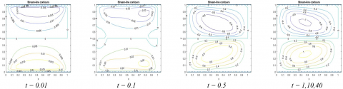
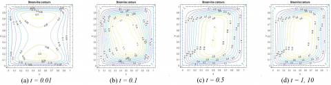
Figures 2 to 5 present the streamline contours for a parallel sided lid-driven cavity problem with different values of Darcy number (Da = 0.01, 0.001) and viscosity ratios (Λ = 1, 3) at various time levels. The streamline contours have different behavior for distinct viscosity ratios at Da = 0.01. Figure 2 depicts the streamline contours for Darcy number Da = 0.01 and viscosity ratio Λ = 1 at distinct time levels. The streamline contours attain an elliptic shape near the horizontal walls of the cavity at time level t = 0.01. The two small circular type contours are generated near the left and right wall of the cavity, inside a single contour of absolute value 0.1 at t = 0.1. The four contours are formed about the horizontal and vertical line through the mid of the cavity at t = 0.5. As time increases from t = 0.5 to 1, the two small contours on the diagonal corner along with a large circular contour with centre at (0.5, 0.5) are developed. This large circular contour moves in an anti-clockwise direction. With an increment of time t = 1 to 2.6, the weaker top-diagonal contour starts expanding (with a clockwise rotation) and shifting the large anti-clockwise rotating contour towards the right vertical wall. And finally, the clockwise rotating contour occupies the whole cavity with two weaker contours in the anti-diagonal corner of the cavity at time level t = 2.7.

The weaker contour in the left-bottom corner of the cavity starts expanding with an anti-clockwise rotation and vanishing the larger clockwise rotating shape with an increment of time t = 2.7 to 5.2. The streamline contours attain the same position as it was at the time level of t = 1. This occupying and vanishing the clockwise or anti-clockwise rotating shapes continue as time increases due to the oscillating behavior in the average Nusselt number at Da = 0.01 (see Figure 10).

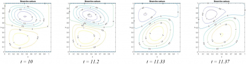
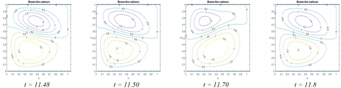
Figure 3 illustrates the streamlined contours for Da = 0.01 and viscosity ratio (Λ = 3) at different time levels. The streamline contours of viscosity ratio (Λ = 3) are similar to Λ = 1 at time t = 0.01, but the intensity of the streamline contours are higher than that of Λ = 1. At t = 0.1, the innermost streamline contours regarding the mid-horizontal line through the geometric centre of the cavity look like a human foot as it has a depression. The streamline contours above the geometric centre of the cavity have a clockwise rotation. In contrast, it has an anti-clockwise rotation in the bottom half of the cavity. It attains a nano-car structure as time increases 0.5 to 1. This behavior retains till time level t = 7.8, and then it starts changing its behavior as time increases. As time increases t = 10 to 11.2, the clockwise rotating elliptic streamline contours dominate the anti-clockwise rotating contours present in the lower half of the cavity. The streamline contours in the lower half of the domain start expanding and shifts the clockwise streamlined contours in the top left corner of the cavity as time increases from 11.33 to 11.37. With an increment in time t = 11.37 to 11.48, the clockwise rotating streamlined contours start dominating the anti-clockwise one in the lower half of the cavity. This process continues as time increases due to the periodicity of the average Nusselt number for Da = 0.01 and Λ = 3 (see Figure 10).

2a.png

2b.png

2c.png

Figure 2. Streamline contours for two-sided lid-driven square porous cavity with Da = 0.01 and Λ = 1

3a.png

3b.png

3c.png

Figure 3. Streamline contours for two-sided lid-driven square porous cavity with Da = 0.01 and Λ = 3

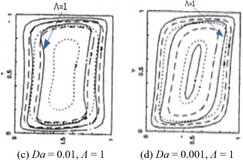
Figures 4 and 5 show the streamline contours for Da = 0.001 with viscosity ratios Λ = 1 and Λ = 3 respectively. The streamline contours for Λ = 1 and Λ = 3 are having a similar behavior at a particular time level t = 0.01, 0.1, 0.5, 1, 10. The streamlined contours about the horizontal centerline of the cavity are elliptic. They have a bend towards the mid of the right vertical wall of the domain for both the viscosity ratio Λ = 1, 3. The difference is in the magnitude of the stream function ψ. The absolute value of stream function ψ decreased with an increase of viscosity ratio Λ = 1 to 3 and a decrease of Darcy number from Da = 0.01 to 0.001.

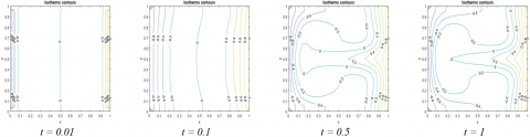
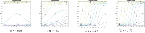
The isotherm contours for different values of Darcy number (Da = 0.01,0.001), viscosity ratio (Λ = 1, 3) at different time levels are presented in Figures 6 to 9. The isotherm contours shift towards the cavity's midpoint with an increment of time t = 0.01 to 0.1. These contours settle near the domain's boundary at time t = 1. As time increases from 1 to 2.6, the isotherm contours occupy almost the whole cavity except the middle part of the lower half of the domain. The left-half region of the cavity contains cold profiles, while the other half includes the hot one. With an increment of time from 2.6 to 4.5, the cold isotherm contours start occupying the whole cavity by pushing the hot isotherms towards the right wall. The contours occupy a ψ type structure and leave the top middle region of the domain at t = 4.7. Further, as time increases 4.7 to 5.2, isotherm contours attain the same structure as a case of time t = 1. Now, this process continues again and again due to the periodicity of the average Nusselt number.

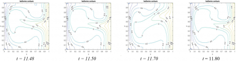
Figure 7 depicts the isotherm contours for Da = 0.01 and Λ = 3 at different time levels. The isotherm contours are symmetric about the horizontal line in the mid of the cavity at t = 0.5. The temperature profiles shifts from the hot (right) wall to the cold (left) wall in an electric bulb-like structure. The cold isotherm from the left vertical wall moves along the top and bottom's mid-wall. While the hot isotherm contours move towards the left wall from the middle of the right wall at t = 0.5 and 1. This position shifts upward along the right boundary as time increases from 1 to 11.20. Further, it tends anti-diagonally as time rises from 11.20 to 11.37. These contours start changing their position to the original one (at t = 1), and then it oscillates between two shapes (that occurred at a time level 1 and 11.37) as time increases.

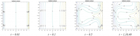
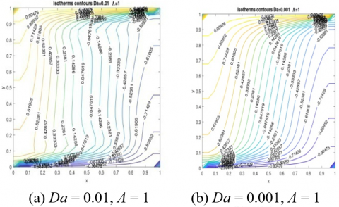
Figures 8 and 9 show the isotherm contours for Da = 0.001 with viscosity ratio Λ = 1 and 3 at distinct time levels. The isotherm contours behave like that of Da=0.01, Λ = 3 till time t = 1 and then attain its steady state. Figures 8 and 9 depict that the cold isotherm contours occupy the region near the left, top, and bottom wall of the cavity from t = 0.5 onwards for both viscosity ratios 1 and 3, Da = 0.001. In contrast, the hot isotherm contours occupy the area near the right boundary and the middle part of the domain as a Conical Flask placed vertically at time level 0.5 and then attain a test-tube structure.

Figures 10 and 11 present the average Nusselt number along the left and right wall of the cavity for different values of Darcy number (Da = 0.01,0.001) and viscosity ratio (Λ = 1, 3). Figure 10 illustrates the average Nusselt number at both left and right wall oscillate periodically after t = 2 with a period of 2.06 for the viscosity ratio Λ = 1 and Da = 0.01. While for Λ = 3, the average Nusselt number at both side walls first attains a steady-state (at approximately t = 1) and then starts oscillating with a minor frequency till 11.206. This frequency enlarges after 11.206 and attains a steady oscillating behavior with a period of 0.29. Figure 11 shows that the average Nusselt number at both sides has the same behavior for both the viscosity ratio Λ = 1 and 3, at Da = 0.001. The average Nusselt number at the left (or right) wall first decrease, then increases, again decreases, and settles steady-state solution at t = 1.25. The numerical simulations were carried out till time level 40 and found it attains steady-state solutions after t = 1.25.

4.png

Figure 4. Streamline contours for two-sided lid-driven square porous cavity with Da = 0.001 and Λ = 1

5.png

Figure 5. Streamline contours for two-sided lid-driven square porous cavity with Da = 0.001 and Λ = 3

6a.png

6b.png

6c.png

Figure 6. Isotherms contours for two-sided lid-driven square porous cavity with Da = 0.01 and Λ = 1

7a.png

7b.png

7c.png

Figure 7. Isotherms contours for two-sided lid-driven square porous cavity with Da = 0.01 and Λ = 3

8.png

Figure 8. Isotherms contours for two-sided lid-driven square porous cavity with Da = 0.001, Λ = 1

9.png

Figure 9. Isotherms contours for two-sided lid-driven square porous cavity with Da = 0.001, Λ = 3

10.png

Figure 10. Average Nusselt-Number for a two-sided lid-driven square porous cavity with Da = 0.01, Λ = 1 and 3, at the left and right wall

11.png

Figure 11. Average Nusselt-Number for a two-sided lid-driven square porous cavity with Da = 0.001, Λ = 1 and 3, at left and right wall

6.2 Case: 2

In this subsection, we will discuss the numerical results for Case 2, in which all the four walls of the cavity are kept moving. The top, bottom, and left, the right walls move with a uniform velocity from left to right, right to the left and top to down, down to the top, respectively. The top and bottom walls are maintained at constant temperature T = 1 and -1, respectively. The heat flux is provided at the left and right walls of the cavity.

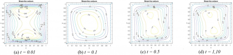
The streamline contours for Darcy number Da = 0.01, 0.001 and viscosity ratio Λ = 1, 3, are depicted in Figures 12 and 13 at different time levels. The two streamline contours are formed one above and the other below the geometric centre of the cavity at t = 0.01. These contours reduce to a single circular contour with some inclination towards the diagonal of the cavity at t = 0.1. The two small contours inside large contours are generated as time increases from t = 0.1 to 0.5. These contours reduce their sizes with an increment of time and attain a steady-state at t = 1 onwards. The inclination of the streamline contours towards the diagonal is greater for Λ = 1 in comparison to Λ = 3.

Figures 14 and 15 show two streamline contours are generated about the geometric center of the square cavity at t = 0.01. These two contours take a peanut-like shape with bends diagonally at t = 0.1. The streamline contours are arranged almost perpendicular to the horizontal axis as time increased from t = 0.1 to 0.5 and attained steady-state. The stream function $\psi$ decreases with increasing viscosity ratio Λ = 1 to 3 for Darcy number Da = 0.01 and 0.001. The stream function $\psi$ decreases with decreasing Darcy number from Da = 0.01 to 0.001 at a particular viscosity ratio.

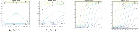
Figures 16 to 19 present the isotherm contours for different values of Darcy number (Da = 0.01,0.001) and viscosity ratios Λ = 1 and Λ = 3 at different time level t = 0.01, 0.1, 0.5, 1 and 10. Figures 16 and 17 show that the isotherm contours are straight lines near the top and bottom walls of the cavity at t = 0.01. The isotherm contours of the top wall shift towards the cavity's left wall at t= 0.1 while contours of the bottom wall shift towards the right wall. The maximal temperature between the top and bottom walls increases from 0 to 0.2 as time changes from 0.01 to 0.1. In the middle of the cavity, isotherm contours bend sharply for viscosity ratio Λ = 1 in comparison to Λ = 3. As time changes from 0.1 to 0.5, isotherm contours from the bottom wall increases then decreases and again increases to approach the top wall for both viscosity ratio (Λ = 1, 3). The effect of viscosity ratio is negligible after t = 0.5 onwards. The isotherm contours attain their steady-state solution after t = 0.5.

Figures 16 to 19 illustrate that the isotherm contours behave almost the same for Darcy numbers Da = 0.01 and 0.001. The variation in contours becomes negligible for Λ = 1, 3 at Da = 0.001. At t = 0.5, isotherm contours increase smoothly from the bottom wall to approach the top wall.

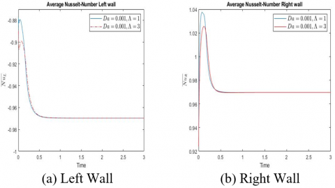
Figures 20 and 21 present the average Nusselt number along the left and right wall of the cavity for different values of Darcy number (Da = 0.01, 0.001) and viscosity ratio Λ = 1 ,3. The average Nusselt number at the left (or right) wall has the same behavior for both viscosity ratio Λ = 1 and 3, at a particular Darcy number. Figure 20 shows that the average Nusselt number at the left (or right) wall first increases, then decreases, and finally attains steady solution for both viscosity ratios Λ = 1 and 3.

Figure 21a shows that the average Nusselt number at the left wall first decreases then increases and again decreases to attain the steady-state solution for both viscosity ratios Λ = 1 and 3, at Da = 0.001. The average Nusselt number at the right wall was first raised then reduced to achieve a steady-state solution (see Figure 21b).

12.png

Figure 12. Streamline contours for four-sided lid driven square porous cavity with Da = 0.01, Λ = 1

13.png

Figure 13. Streamline contours for four-sided lid driven square porous cavity with Da = 0.01, Λ = 3

14.png

Figure 14. Streamline contours for four-sided lid driven square porous cavity with Da = 0.001, Λ = 1

15.png

Figure 15. Streamline contours for four-sided lid driven square porous cavity with Da = 0.001, Λ = 3

16.png

Figure 16. Isotherms contours for four-sided lid driven square porous cavity with Da = 0.01, Λ = 1

17.png

Figure 17. Isotherms contours for four-sided lid driven square porous cavity with Da = 0.01, Λ = 3

18.png

Figure 18. Isotherms contours for four-sided lid driven square porous cavity with Da = 0.001, Λ = 1

19.png

Figure 19. Isotherms contours for four-sided lid driven square porous cavity with Da = 0.001, Λ = 3

20.png

Figure 20. Average Nusselt-Number for a four-sided lid-driven square porous cavity with Da = 0.01, Λ = 1 and 3, at left and right wall

21.png

Figure 21. Average Nusselt-Number for a four-sided lid-driven square porous cavity with Da = 0.001, Λ = 1 and 3, at left and right wall

The average Nusselt number at the left (right) wall decrease with an increase of viscosity ratio from Λ=1 to 3 for both the Darcy number (Da = 0.01, 0.001). It also decreases with a decrease of Darcy number from Da = 0.01 to 0.001 at a particular viscosity ratio (Λ = 1 and 3).

This paper investigates the mixed convection inside a two-sided and four-sided lid-driven square cavity filled with porous media. We have employed the finite difference method to calculate the numerical solutions. We have compared our present results with the particular case in which all four walls of the cavity are stationary with previously published work and found to be in good agreement. We can conclude the following points from the current study.

Case 1: Two-sided lid-driven square cavity

1. The absolute value of ψ decreases with an increase of viscosity ratio Λ = 1 to 3 and a decrease of Darcy number Da = 0.01 to 0.001.

2. The viscosity ratio has a significant role in the numerical computation of isotherm contours at Da = 0.01. The effect of viscosity ratio Λ = 1, 3 is negligible with decreasing of Darcy number Da = 0.01 to 0.001.

3. The average Nusselt number at the left and right wall has oscillating behavior for Da = 0.01 with viscosity ratio Λ = 1 and 3. The average Nusselt number at the left and right wall for Λ = 3 attains an approximate steady-state solution at t = 1.25.

Case 2: Four-sided lid-driven square cavity

1. The stream function ψ decreases with an increasing of viscosity ratio Λ = 1 to 3 and a decreases of Darcy number from Da = 0.01 to 0.001.

2. The absolute value of average Nusselt number at left (or right) wall decrease with an increase of viscosity ratio from Λ = 1 to 3 and a decreasing of Darcy number from Da = 0.01 to 0.001.