Youkun Zhong
© 2021 IIETA. This article is published by IIETA and is licensed under the CC BY 4.0 license (http://creativecommons.org/licenses/by/4.0/).
OPEN ACCESS
With the technical development of energy conservation and emission reduction technology, the internal structure of engineering machinery has become denser. The rising full-machine heat load that ensues challenges the effect of the cooling system. In the traditional thermal management system for the transmission in energy machinery, the cooling capacity does not fully match the load of each subsystem, and the thermal management components cannot adapt to the dynamic cooling demand of engineering machinery. To solve these problems, this paper designs and analyzes the thermal management system of power matching transmission in energy machinery. Firstly, the energy distribution among different components of engineering machinery, including, hydraulic system, transmission system, and cooling system, was described in each work section, and the dynamic matching method was detailed for hydraulic torque converter. Then, heat source engine, hydraulic torque converter, and hydraulic retarder were selected as the targets of thermal management for the power transmission system of loader. Next, the thermal management cycle was framed as a scheme in which the engine transmission system is independent with the cooling circulation system, and a heat transfer calculation model was constructed for loader transmission system. The proposed model was proved effective through experiments. The research results provide a reference for the thermal management of other subsystems of engineering machinery.
engineering machinery, power matching, transmission, thermal management design
Engineering machinery has aroused widespread attention in the society, as an important part of basic construction equipment and equipment industry. Despite its rapid development, engineering machinery faces several noneligible problems: high energy consumption, low operating efficiency, and excessive heat loss. These problems are inevitable due to the late start of research into engineering machinery. Hence, the energy conservation and emission reduction raise a growing concern in the industry [1-4].
The installation of auxiliary energy-saving devices increases the internal density of engineering machinery. The rising full-machine heat load that ensues challenges the effect of the cooling system [5-8]. To enhance the full-machine performance in dynamics, economy, and greenness, it is important to carry out energy analysis, power matching, and full-machine thermal management of engineering machinery, especially loader.
Under the premise of ensuring the speed control and overload capacity of engineering machinery, replacement engine with motor is an effective way to realize an energy-efficient, low-emission drive mode [9-10]. To improve the energy efficiency, operability, dynamics, and safety of the full machine, it is of great significance to study the power matching structure and control strategy of engineering machinery under complex conditions [11-14]. Wang et al. [15] analyzed the load features and working conditions of the hydraulic excavator driven by permanent magnet synchronous motor, put forward a power assembly parameter matching method that improves the full-machine performance, and provided a variable pressure difference control strategy suitable for low-speed small flows. To improve the performance of wheel loader transmission system, Niu et al. [16] constructed a dynamic simulation model of loader transmission system to reduce fuel consumption in each cycle and heat generation, optimized the main parameters of loader transmission by genetic algorithm (GA), and examined the influence of different flow modes on the flow field inside the oil cooler, in view of the cooling demand of the transmission system. Using the performance calculation method based on heat transfer units (HTUs), Wang et al. [17] investigated the relationship between the surface air flow rate and air-side resistance of the radiator of engineering machinery, clarified the method for cooling fan selection and the design steps of variable circulation, and designed a full-machine thermal balance test, revealing that the prototype with two circulating cooling systems has relatively low energy consumption. To prevent the overheating and overcooling of engineering machinery, Nguyen et al. [18] selected the main components and discussed the control strategy for the electronically controlled hydraulic fan cooling system based on BODAS controller, and evaluated the energy efficiency of the cooling system by measuring and comparing the heat release of the system and the economy of the engine.
Heat dissipation is needed for both the engine of engineering machinery and the hydraulic oil of hydraulic torque converter. The huge cooling demand cannot be satisfied with one cooling fan alone [19-22]. Naumenko et al. [23] carried out the matching design for the cooling fan and radiator of engineering machinery, reconfigured the thermal parameters and component parameters of the hydraulic drive and transmission, and conducted experiments to compare the engine water temperatures and preheating times before and after system improvement; their electro-hydraulic hybrid drive cooling system was proved effective in cooling.
In the traditional thermal management system for the transmission in energy machinery, the cooling capacity does not fully match the load of each subsystem, and the thermal management components cannot adapt to the dynamic cooling demand of engineering machinery. To solve these problems, this paper designs and analyzes the thermal management system of power matching transmission in energy machinery. The target engineering machinery is a loader. Section 2 analyzes the energy distribution among different components of engineering machinery, including, hydraulic system, transmission system, and cooling system in each work section, and provides a dynamic matching method for hydraulic torque converter. Section 3 determines the targets of thermal management for the power transmission system of loader: heat source engine, hydraulic torque converter, and hydraulic retarder, prepares as a scheme in which the engine transmission system is independent with the cooling circulation system, takes the scheme as the framework of the thermal management cycle, and constructs a heat transfer calculation model for loader transmission system. The proposed model was proved effective through experiments.
The target engineering machinery is a loader that operates under two conditions: loading and transportation. Each cycle of the loading operation consists of five work sections, namely, forwarding, reversing, shoveling, unloading-forwarding-lifting, and zero-load reversing. This section carries out data analysis on the work features of the loader in each work section. Table 1 presents the highest speed, average speed, transport distance, and work time of each work section.
Table 1. Information of loader operation in each work section
|
Items |
Work section 1 |
Work section 2 |
Work section 3 |
Work section 4 |
Work section 5 |
|
Highest speed |
2.11 |
2.31 |
0.65 |
2.81 |
2.15 |
|
Average speed |
1.43 |
1.47 |
0.24 |
1.37 |
1.65 |
|
Transport distance |
12.3 |
13.2 |
1.35 |
12.3 |
12.5 |
|
Work time |
8.1 |
9.4 |
6.2 |
8.8 |
7.3 |
2.1 Subsystem energy distribution
The hydraulic steering system of the loader adopts a control method that combines dual pump converging with load sensing. Let F, L and P be the working pressure, flow, and working efficiency of hydraulic components, respectively. According to the oil pressure and engine speed signals measured by pressure and speed sensors, the power of each hydraulic component in the system can be calculated by:
$\omega_{p}=\frac{F \cdot L \cdot P}{60}$ (1)
The power calculated by formula (1) reflects the energy allocated to each component of the hydraulic system in each work section (Table 2). During the shoveling, the loader needs to allocate some power to the working pump and the steering pump. In this work section, the working efficiency of the hydraulic system is as high as 68%. The other sections witness a low working efficiency and a high energy consumption. During forwarding, reversing, and zero-load reversing, more power is allocated to the steering pump than to the working pump.
The output power of the loader engine equals the sum of the output powers of every hydraulic pump and hydraulic torque converter. Figure 1 presents the structure of hydraulic torque converter. Let ω be the total output power of engine; Σωp be the sum of engine powers consumed by hydraulic pumps. Then, the input power of hydraulic torque converter can be calculated by:
$\omega_{T}=\omega-\sum \omega_{p}$ (2)
Let ZJ1 and ZJ2 be the input torques of the front and rear drive bridges of the engine, respectively; rI be the input speed of the gearbox, which equals the turbine speed of hydraulic torque converter; it and Pt be the transmission ratio and transmission efficiency of gearbox, respectively. Then, the input power of gearbox can be calculated by:
$\omega_{V}=\frac{\left(Z J_{1}+Z J_{2}\right) r_{I}}{9550 i_{t} P_{t}}$ (3)
Table 3 shows the energy allocation of loader transmission in each work section. In each operational cycle, the transmission system has an average efficiency of merely 65%. To lower the heat generation of the system to 28.46kW, the engine’s output power must surpass 72%. The variable speed pump has smaller average power than other working components.
Figure 1. Structure of hydraulic torque converter
Table 2. Energy allocation to each component of the hydraulic system in each work section
|
Hydraulic components |
Work section 1 |
Work section 2 |
Work section 3 |
Work section 4 |
Work section 5 |
|
Heat loss |
8.35 |
16.91 |
14.75 |
11.95 |
11.85 |
|
Working pump |
3.76 |
9.82 |
27.61 |
20.13 |
2.79 |
|
Steering Pump |
7.53 |
17.37 |
13.58 |
14.36 |
12.61 |
|
Rotating bucket cylinder |
0 |
0 |
9.55 |
4.12 |
0 |
|
Boom cylinder |
0 |
7.65 |
13.98 |
17.39 |
0 |
|
Steering cylinder |
2.41 |
3.41 |
0.96 |
1.65 |
3.25 |
|
Efficiency |
21.73 |
41.61 |
60.55 |
65.82 |
22.63 |
Table 3. Energy allocation of components in loader transmission in each work section
|
Transmission components |
Work section 1 |
Work section 2 |
Work section 3 |
Work section 4 |
Work section 5 |
|
Heat loss |
21.98 |
39.52 |
48.65 |
17.66 |
27.82 |
|
Gearbox |
31.75 |
55.31 |
32.79 |
52.37 |
25.49 |
|
Variable speed pump |
1.24 |
1.27 |
1.32 |
1.35 |
1.02 |
|
Hydraulic torque converter |
53.57 |
96.41 |
79.25 |
71.92 |
50.37 |
|
Total output of engine |
71.85 |
123.67 |
116.31 |
103.08 |
62.53 |
|
Efficiency |
63.72 |
57.39 |
42.50 |
75.21 |
51.13 |
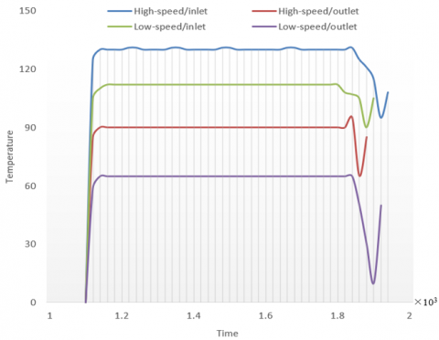
The cooling system discharges the heat generated by the hydraulic system and the transmission system to the outside of the engine compartment in two modes: self-dissipation and radiator dissipation. Let σo and φo be the specific heat at constant pressure and density of the oil, respectively; ∆T be the inlet-outlet temperature difference of the radiator. Based on the signal measured by temperature sensors, the cooling power of each radiator in the loader system under heat balance can be calculated by:
$\omega_{C}=\frac{\sigma_{o} \varphi_{o} L \Delta T}{60}$ (4)
The energy allocation in the cooling system of the loader can be derived from the cooling power obtained by formula (1). Figure 2 presents the inlet and outlet temperature curves of each radiator. During the shoveling operation, the temperatures of transmission oil and hydraulic oil of the loader both increase with fluctuations. The transmission system loses more energy, and operates at a lower efficiency (55%) than the hydraulic system. In the hydraulic system, the heat loss is dissipated by components like radiators. In the transmission system, the heat loss is dissipated with the aid of gearbox housing and transmission oil. After the full machine reaches heat balance, the thermal performance should be optimized if the transmission oil is still too hot.
Figure 2. Inlet and outlet temperature curves of each radiator
2.2 Dynamic matching of hydraulic torque converter
Let ZJO be the output torque of the engine. The engine torque consumed by each hydraulic pump can be calculated by ZJp=FL/2πP, and the sum of torques can be expressed as ∑ZJp. Then, the input torque of hydraulic torque converter can be calculated by:
$Z J_{\omega}^{A}=Z J_{O}-\sum Z J_{p}$ (5)
Table 4 shows the allocation of engine torque in the five work sections during shoveling operation. The allocation varies from section to section, due to the large difference between main components, such as torque converter, steering pump, working pump, and variable speed pump, in working stability.
Table 4. Allocation of engine torque in the five work sections
|
Sections |
Work section 1 |
Work section 2 |
Work section 3 |
Work section 4 |
Work section 5 |
|
|
Output torque |
435.10 |
417.31 |
647.25 |
454.87 |
405.82 |
|
|
Torque converter |
Mean |
359.03 |
172.73 |
364.49 |
165.31 |
275.48 |
|
Proportion |
81.21 |
42.32 |
55.96 |
42.05 |
68.35 |
|
|
Variable speed pump |
Mean |
9.58 |
8.75 |
11.56 |
9.68 |
8.76 |
|
Proportion |
2.29 |
2.08 |
1.52 |
2.16 |
2.05 |
|
|
Steering pump |
Mean |
51.71 |
155.72 |
115.66 |
115.92 |
92.62 |
|
Proportion |
11.35 |
34.27 |
16.05 |
23.52 |
25.34 |
|
|
Working pump |
Mean |
23.81 |
83.59 |
176.82 |
123.24 |
21.37 |
|
Proportion |
5.23 |
21.54 |
26.67 |
31.73 |
5.17 |
|
To stabilize the circulating flow of the dynamic liquid in hydraulic torque converter, it is necessary to keep the inlet and outlet oil pressures stable during loader movement. Let NJBAL and NJEAL be the dynamic liquid torques on the pump wheel shaft and the turbine shaft, respectively; NJBA and NJEA be the dynamic torques on the pump wheel shaft and the turbine shaft, respectively; JB and JE be the rotational inertias between pump wheel and pump wheel shaft, and between turbine and turbine shaft, respectively; AVB and AVE be the angular velocities of pump wheel and turbine, respectively. Then, the torque of the working hydraulic force for the hydraulic torque converter can be expressed as:
$\left\{\begin{array}{l}N J_{B}^{A L}=N J_{B}^{A}-J_{B} \frac{d A V_{B}}{d t} \\ N J_{E}^{A L}=J_{E}^{A}-J_{E} \frac{d A V_{E}}{d t}\end{array}\right.$ (6)
Let l, PL, μL, and iL be the torque ratio, torque efficiency, moment efficiency, and transmission ratio, respectively. Then, the relationship between them can be fitted by least squares method:
$\left\{\begin{array}{l}\mu_{L}=-5.45 i_{L}^{3}+3.49 i_{L}^{2}+0.73 i_{L}+3.32 \\ l=-2.29 i_{L}^{3}+1.12 i_{L}^{2}-1.671 i_{L}+2.46 \\ P_{L}=-2.68 i_{L}^{2}-1.54 i_{L}-0.01\end{array}\right.$ (7)
Formula (7) shows that AVB, AVE, JB, and JE greatly influence the dynamic features of hydraulic torque converter. Then, the output torque of turbine axle can be derived from the transmission shaft torque measured by torque sensor:
$N J_{E}^{A}=\frac{Z J_{1}+Z J_{2}}{i_{t} P_{t}}$ (8)
Based on formula (6) and the angular acceleration curve of hydraulic torque converter, the dynamic torque ratio of hydraulic torque converter can be calculated by:
$l=\frac{N J_{E}^{A L}}{N J_{B}^{A L}}$ (9)
The dynamic mathematical model of hydraulic torque converter can be expressed as:
$\left\{\begin{array}{l}i_{L}=A V_{E} / A V_{B} \\ l=\frac{N J_{E}^{A L}+J_{E} \frac{d A V_{E}}{d t}}{N J_{B}^{A L}+J_{B} \frac{d A V_{B}}{d t}} \\ P_{L}=i_{L} l\end{array}\right.$ (10)
When the hydraulic torque converter works stably, the inertia resistance moments of the turbine and pump wheel speeds are zero. Let l* be the static torque ratio of hydraulic torque converter. Then, there exists JEdAVE/dt=JBdAVB/dt=0, and NJEA= l*×NJBE. Then, the dynamic torque ratio in formula (10) can be transformed into:
$l=l^{*}+\frac{l^{*} J_{B}+i_{t} J_{E}}{N J_{B}^{A} / \frac{d A V_{B}}{d t}-J_{B}}$ (11)
As can be seen from formulas (7) and (11), when the transmission ratio it remains unchanged, the l value first increases and then declines with the growth of AVB; the l value first decreases and then rises with the decline of AVB. Thus, under a relatively large dAVB/dh, the l value fluctuates about l=l1-((l1JB+iLJE)/JB. This law is consistent with the previous analysis, and the efficiency PL of hydraulic torque converter follows the same change pattern as l.
The thermal management of loader transmission has three targets: heat source engine, hydraulic torque converter, and hydraulic retarder. There are two schemes for thermal management cycle. In the first scheme, the engine transmission and cooling circulation systems are coupled; in the second schemes, the two systems are independent of each other. On the upside, the first scheme boasts a compact thermal management system, and low efficiency of secondary heat transfer; on the downside, the system is too complicated to be maintained at a low cost. The second scheme features a simple structure, reliable operations, and a high cooling efficiency. Besides, the weak coupling between control variables makes it easy to implement the control strategy. To rationalize the control system of thermal management system, this paper decides to study the dynamic transmission system and thermal management system separately, i.e., adopt the second scheme to analyze the thermal load and thermal performance of the two systems (Figure 3).
Figure 3. Working principle of Scheme 2
This section aims to model the structure of the thermal management system for loader engine, which consists of water jacket, water pump, thermostat, radiator, expansion tank, and heater. In the thermal management system, the power and temperature cycle of the engine are respectively controlled by water pump and thermostat. The radiator is responsible for the heat exchange between the engine and the environment after the start of the cooling cycle. The pressure stability of the system is mainly achieved by bubble discharge of the expansion tank. Let SCL be the equivalent cross-sectional area of the cooling pipe; ∆F be the inlet-outlet pressure difference of the coolant of the heat management component; φC be the density of the coolant. Then, the volumetric flow LV of the engine’s heat management component can be described by modified Bernoulli’s equation:
$L_{V}=S_{C L} \cdot \sqrt{\frac{2 \cdot \Delta F}{\varphi_{C}}}$ (12)
Let ETAH be the heat exchange amount between the engine housing and the cooling pipe; υM and ωM be the engine speed and the corresponding maximum power. Then, the heat exchange amount between the engine and the coolant can be calculated by:
$E_{T A H}=g\left(v_{M}, \omega_{M}\right)$ (13)
Let σM and EU be the heat capacity unit of the cooling pipe and the resistance unit of the system, respectively; FM and TψM be the pressure and temperature of the hot fluid passing through the heat capacity unit, respectively; DM be the volume of the cooling pipe of the engine; dE be the heat entering that volume; σF be the specific heat of the fluid, which depends on the fluid’s working pressure and temperature; φC be the fluid density. Then, the differentials of TM and FM relative to time, denoted respectively as dTM/dt and dFM/dt, must satisfy:
$\frac{d T_{M}}{d t}=\frac{d E}{\sigma_{F} \cdot \varphi_{C} \cdot D_{M}}+\frac{d T_{M}}{\varphi_{C} \sigma_{F}} \cdot \frac{d F_{M}}{d t}$ (14)
Let dqe1, dqe2 and dq1, dq2 be the heat flow and mass flow entering the heat capacity unit of the cooling pipe; de be the heat exchange amount between the heat capacity unit and the environment; e be the heat of the fluid in the unit. Then, dE can be calculated by:
$d E=d q e_{1}+d q e_{2}+d e-\left(d q_{1}+d q_{2}\right) \cdot e$ (15)
Let dφFbe the variation of density; δ and β be the elastic modulus and volume expansion coefficient of the liquid, respectively. Both δ and β depends on the working pressure and temperature of the medium. Then, the pressure per unit volume can be described by the following differential equation:
$\frac{d F_{M}}{d t}=\delta \cdot \frac{d \varphi_{E}}{\varphi_{E}}+\delta \cdot \beta \cdot \frac{d T_{M}}{d t}$ (16)
The inlet/outlet mass flow dq' and heat flow dq'·e' of the resistance unit of the engine can be derived based on the resistance unit of the cooling system. Assuming that the inlet and outlet heat flows are equal for each resistance unit, dq' can be calculated as by:
$d q^{\prime} e_{1}^{\prime}=d q^{\prime} \cdot e_{1}^{\prime}$ (17)
$d q^{\prime} e_{2}^{\prime}=d q^{\prime} \cdot e_{1}^{\prime}$ (18)
The cooling system of the engine is powered by the centrifugal water pump driven at a fixed speed by the crankshaft of the engine. Let υM be the speed of the engine; iP/M be the speed ratio of the cooling water pump to the engine. Then, the speed of the cooling water pump can be calculated by:
$v_{W P}=v_{M} \cdot i_{P / M}$ (19)
The displacement and speed of the cooling water pump determine its inlet-output pressure difference. The fluid temperature at the outlet of the water pump can be obtained from the measured temperature of the inlet fluid and the calculation results on the pump’s work on the fluid. Here, the cooling water is treated as an ideal incompressible fluid. Let γa be the convection coefficient between coolant and oil; σW be the heat capacity of the oil; TEC be the coolant temperature at the inlet of the thermostat. Then, the power of the water pump can be calculated by:
$\frac{d T_{W P}}{d t}=\frac{\gamma_{a}}{\sigma_{W}} \cdot\left(T_{E C}-T_{W P}\right)$ (20)
The flow regime of coolant depends on the Reynolds number. For the water-air radiator, the volumetric flow of the coolant can be determined by the inlet and outlet pressures, and used to deduce the rated heat exchange amount of the radiator. The heat exchange amount between the radiator and the coolant can be characterized by the function between the volumetric flow of coolant and the mass flow of the air. The relationship between the inlet temperature TEHS, outlet temperature TOHS, and inlet-outlet temperature difference dTHS of the radiator can be described as:
$d T_{H S}=T_{E H S}-T_{O H S}$ (21)
Let ψEact, ψOact, and EHS be the measured inlet temperature, measured outlet temperature, and heat release of the radiator, respectively; PHS be the thermal efficiency of the radiator. Then, the actual heat release Eact of the radiator can be calculated by:
$E_{a c t}=E_{H S} \cdot\left(T_{\text {Eact }}-T_{\text {Oact }}\right) / d T_{H S} \cdot P_{H S}$ (22)
The cooling effect of the radiator differs significantly between ventilation area and non-ventilation area. To calculate the total heat exchange amount of the radiator, it is necessary to compute the heat exchange amounts of the two areas, both of which are related to air flow rate. Let υNT, and υAFR be the air flow rates before and after the radiator fans are opened; υOA be the additional wind speed brought by the fan. Then, we have:
$v_{A F R}=v_{N T}+v_{O A}$ (23)
Ignoring the air flow at the center of the radiator fans, the overall mapping area SFMA of the fan can be obtained by adding up the actual coverage of the fan with the rotational area at the center of the fan. Let ONfan and INfan the outer and inner diameters of the fan, respectively. Then, the SFMA value can be calculated by:
$S_{F M A}=\frac{\pi}{4}\left(O N_{f a n}^{2}-I N_{f a n}^{2}\right)$ (24)
Let Ф and U be the length and height of the radiator, respectively. Then, the non-mapping area of the fan SNFMA can be calculated by:
$S_{N F M A}=\Phi \cdot U-S_{F M A}$ (25)
Suppose the heat exchange amount of the radiator is determined by the air flow rate in the mapping area and the volumetric flow of the coolant. The functional relationship between the two determinants can be illustrated as g(υFMA, LR). Then, the heat exchange amount EFMA within SFMA can be expressed as:
$E_{F M A}=g\left(v_{F M A} \cdot L_{R}\right) \cdot \frac{S_{F M A}}{\Phi \cdot U}$ (26)
Suppose the heat exchange amount of the radiator is determined by the air flow rate in the non-mapping area and the volumetric flow of the coolant. The functional relationship between the two determinants can be illustrated as g(υNT, LR). Then, the heat exchange amount ENFMA within SNFMA can be expressed as:
$E_{N F M A}=g\left(v_{N T} \cdot L_{R}\right) \cdot \frac{S_{N F M A}}{\Phi \cdot U}$ (27)
The total heat exchange amount ET can be obtained by:
$E_{T}=E_{F M A}+E_{N F M A}$ (28)
Let φF and SNG be the density of the working medium and the effective diameter of the driving wheel of hydraulic retarder, respectively; a be the gravity acceleration; μTC and AVG be the braking torque coefficient and the annular velocity of the drive wheel, respectively. Then, the braking torque of hydraulic retarder can be calculated by:
$T_{C}=\varphi_{E} \cdot a \cdot \mu_{T_{C}} \cdot A V_{G}^{2} \cdot S N_{G}^{5}$ (29)
Let QLP and MSL be the heat flow of power loss and braking torque of the retarder, respectively; rM be the engine speed. Since the transmission fluid in the retarder contains much more kinetic energy than the fluid, QLP can be empirically approximated by:
$Q_{L P}=\frac{M_{S L} \cdot r_{M}}{9550}$ (30)
The cyclic flow features of the retarder can be characterized by the effective displacement of the variable pump. Let υED and υFD be the effective displacement and displacement baseline of the variable pump, respectively; ηVPD be the proportional coefficient of the variable displacement of the variable pump. Then, the υED value can be calculated by:
$v_{E D}=v_{F D} \cdot \eta_{V P D}$ (31)
Let LVP and rVP be the volumetric flow and speed of the variable pump, respectively. Then, the rated volumetric flow of the pump can be calculated by:
$L_{V P}=v_{E D} \cdot r_{V P}$ (32)
Under different working speeds, the retarder sees changes in transmission fluid flow, inlet pressure, and output pressure. Any change to the flow in the thermal management system will change the pressure increment of the retarder. Therefore, the proposed thermal management system for the full-machine power transmission system must simulate the correspondence between these changing parameters with a pilot pump. Let fs be the lever position of the retarder. Then, the relationship between the outlet and inlet pressures of the retarder can be defined as:
$F_{O}=F_{I}+f_{s}$ (33)
The selected loader and its hydraulic torque converter have three components and a single turbine. The dynamic features of the loader were analyzed during the maximum power output period, such that the opening of the accelerator pedal remains the same during the experiments. Table 5 presents the experimental results on the dynamic features of hydraulic torque converter. The highest efficiency (0.835) of the hydraulic torque converter was achieved at the transmission ratio of 0.6, the torque coefficient of 1.37, and the engineering torque of 115.
Table 5. Experimental results on the dynamic features of hydraulic torque converter
|
Transmission ratio |
Torque coefficient |
Engineering torque |
Efficiency |
|
0 |
2.505 |
121 |
0 |
|
0.1 |
2.15 |
121 |
0.215 |
|
0.2 |
1.92 |
121 |
0.379 |
|
0.3 |
1.835 |
121.3 |
0.5362 |
|
0.4 |
1.755 |
121.6 |
0.705 |
|
0.5 |
1.56 |
121 |
0.75 |
|
0.6 |
1.37 |
115 |
0.835 |
|
0.7 |
1.1 |
100 |
0.82 |
|
0.8 |
1.05 |
85 |
0.831 |
|
0.9 |
1 |
82 |
0.810 |
|
0.94 |
0.905 |
65 |
0.8205 |
|
0.96 |
0.85 |
50 |
0.7706 |
Figure 4 shows the engine speed curve of the loader during the driving process. Figure 5 presents the lever change curve of the speed converter of the engine. During horizontal movement, the engine speed changed in [1,300r/min, 1,700r/min]; During uphill and downhill movements, the speed converter of the engine was mostly switched to the high lever.
Figure 6 displays the coolant temperature curves under normal driving. The fan was driven by traditional mechanical control with fixed speed ratio, and temperature control. Under either control mode, the coolant temperature at the outlet of the engine tended to be stable after 1,300s. Compared with mechanical control, the temperature control had a low stable temperature and good cooling effect.
During the uphill movement, the loader speed and wind speed were both slow; the fan speed was also slow, due to the constraint of the engine speed. In this case, the coolant temperature rose faster and fluctuated more violently under mechanical control than temperature control.
Figure 4. Engine speed curve
Figure 5. Lever change curve of the speed converter
Figure 6. Coolant temperature curves of engine
Figure 7 shows the mean parasitic power curves of the engine during normal driving. The fan was driven by traditional mechanical control with fixed speed ratio, and temperature control. Throughout the movement, the engine consumed an average of parasitic power of 12.84kW during high-speed downhill movement and low-speed downhill movement, when the cooling fan was under mechanical control. By contrast, a low parasitic power was consumed (4.75kW) when the fan was under temperature control.
For the thermal management of the loader transmission during shoveling, the mechanically controlled fan speed was fixed at 1,350r/min with the retarder in on state. Figure 8 shows the curves of the inlet and outlet temperatures of transmission fluid in the oil-air radiator during the slow movement and shoveling of the loader. Under slow movement, the retarder operated at a slow speed, and the transmission fluid of the radiator worked in the temperature range of [87.6℃, 128.2℃], meeting the work requirements of the fluid. During shoveling, the retarder operated at full load, and the transmission fluid of the radiator worked in the temperature range of [61.4℃, 104.2℃], slightly lower than the working temperature of the fluid.
Figure 9 shows the curves of the inlet and outlet temperatures of transmission fluid in the oil-air radiator with temperature-controlled fans during the slow movement and shoveling of the loader. During shoveling, the working state of the retarder and the transmission fluid temperature were similar to those under mechanical control. Under slow movement, the transmission fluid of the radiator worked in the temperature range of [60.1℃,102.8℃], which is closer to the normal working temperature of the fluid than that under mechanical control.
Figure 7. Mean parasitic power curves of engine
Figure 8. Transmission fluid temperature curves 1 of the radiator with fans under mechanical control
Figure 9. Transmission fluid temperature curves 2 of the radiator with fans under temperature control
Figure 10. Power consumption of fans
Figure 10 compares the power consumptions of fans under mechanical control and temperature control, as the loader moves uphill at high speed and low speed. Under mechanical control, basically the same power was consumed by the loader, as it moved uphill at high speed and low speed. Under temperature control, more power was consumed for high-speed uphill movement (48.1kW) than for low-speed uphill movement (26.4kW).
This paper designs and analyzes the thermal management system of power matching transmission in energy machinery. Firstly, the authors described the energy distribution among different components of engineering machinery, including, hydraulic system, transmission system, and cooling system in each work section, and detailed the dynamic matching method for hydraulic torque converter. After that, the dynamic features of the torque converter were tested, and the engine speed curve throughout the driving process was plotted based on the test results. Then, heat source engine, hydraulic torque converter, and hydraulic retarder were selected as the targets of thermal management for the power transmission system of loader, the scheme in which the engine transmission system is independent with the cooling circulation system was adopted as the framework of the thermal management cycle, and the corresponding heat transfer model was built for the loader transmission. During the experiments, the fans were controlled by two different methods: traditional mechanical control with fixed speed ratio, and temperature control. Under the two control modes, the authors investigated the variations in the coolant temperature of engine, mean parasitic power of engine, transmission fluid temperature of radiator, and the power consumption of radiator fans. The experimental results confirm the effectiveness of our model, and provide a reference for the thermal management of other subsystems of engineering machinery.
Research on the Reform and Practice of Undergraduate Classroom Teaching in Local Colleges and Universities Based on Teaching Efficiency, Guangxi Higher Education Undergraduate Teaching Reform Project in 2019 (Grant No.: 2019JGZ143).
[1] Bonci, M., Begovic, A., Governatori, D., Marchini, D., Vivio, F. (2020). An Analytical Procedure to Analyse Efficiency, Cooling and Thermal Management of a BEV Sport Car Transmission (No. 2020-24-0023).
[2] Heidarzadeh, H., Rostami, A., Dolatyari, M. (2020). Management of losses (thermalization-transmission) in the Si-QDs inside 3C–SiC to design an ultra-high-efficiency solar cell. Materials Science in Semiconductor Processing, 109: 104936. https://doi.org/10.1016/j.mssp.2020.104936
[3] Agarwal, S., Mishra, J.K., Priye, V. (2020). Thermal design management of highly mechanically stable wavelength shifter using photonic crystal waveguide. Superlattices and Microstructures, 142: 106510. https://doi.org/10.1016/j.spmi.2020.106510
[4] Zhang, Y., Jin, Y., Yao, J., Zhu, G., Wen, B. (2017). Power peak shaving with data transmission delays for thermal management in smart buildings. IEEE Transactions on Industrial Informatics, 14(4): 1532-1541. https://doi.org/10.1109/TII.2017.2781256
[5] An, J., Binder, A. (2017). Operation strategy with thermal management of E-machines in pure electric driving mode for twin-drive-transmission (DE-REX). In 2017 IEEE Vehicle Power and Propulsion Conference (VPPC), pp. 1-6. https://doi.org/10.1109/VPPC.2017.8330925
[6] Elqady, H.I., Abo-Zahhad, E.M., Ali, A.Y., Elkady, M.F., El-Shazly, A.H., Radwan, A. (2020). Header impact assessment of double-layer microchannel heat sink in the computational fluid mechanics simulation for CPV thermal management. Energy Reports, 6: 55-60. https://doi.org/10.1016/j.egyr.2020.10.037
[7] Viehhauser, G. (2015). Thermal management and mechanical structures for silicon detector systems. Journal of Instrumentation, 10(9): P09001. https://doi.org/10.1088/1748-0221/10/09/P09001
[8] Gupta, S.K., Kar, K., Mishra, S., Wen, J.T. (2017). Incentive-based mechanism for truthful occupant comfort feedback in human-in-the-loop building thermal management. IEEE Systems Journal, 12(4): 3725-3736. https://doi.org/10.1109/JSYST.2017.2771528
[9] Kim, K.H., Oh, Y., Islam, M.F. (2013). Mechanical and thermal management characteristics of ultrahigh surface area single‐walled carbon nanotube aerogels. Advanced Functional Materials, 23(3): 377-383. https://doi.org/10.1002/adfm.201201055
[10] Wang, Y., Chen, L., Cheng, H., Wang, B., Feng, X., Mao, Z., Sui, X. (2020). Mechanically flexible, waterproof, breathable cellulose/polypyrrole/polyurethane composite aerogels as wearable heaters for personal thermal management. Chemical Engineering Journal, 402: 126222. https://doi.org/10.1016/j.cej.2020.126222
[11] Teh, J., Lai, C.M. (2019). Risk-based management of transmission lines enhanced with the dynamic thermal rating system. IEEE Access, 7: 76562-76572. https://doi.org/10.1109/ACCESS.2019.2921575
[12] Lu, P., Gao, Q., Lv, L., Xue, X., Wang, Y. (2019). Numerical calculation method of model predictive control for integrated vehicle thermal management based on underhood coupling thermal transmission. Energies, 12(2): 259. https://doi.org/10.3390/en12020259
[13] Park, M., Jung, D., Kim, M., Min, K. (2013). Study on the improvement in continuously variable transmission efficiency with a thermal management system. Applied Thermal Engineering, 61(2): 11-19. https://doi.org/10.1016/j.applthermaleng.2013.07.032
[14] Ganesan, S., Subramanian, S. (2012). Non-convex economic thermal power management with transmission loss and environmental factors: Exploration from direct search method. International Journal of Energy Sector Management, 6(2): 228-238. https://doi.org/10.1108/17506221211242086
[15] Wang, J., Tang, X., Zheng, P., Li, S., Zhou, T., Xie, R.J. (2019). Thermally self-managing YAG: Ce–Al2O3 color converters enabling high-brightness laser-driven solid state lighting in a transmissive configuration. Journal of Materials Chemistry C, 7(13): 3901-3908. https://doi.org/10.1039/C9TC00506D
[16] Niu, W., Zhang, L., Wang, Y., Wang, Z., Zhao, K., Wu, S., Tok, A.I.Y. (2019). Multicolored photonic crystal carbon fiber yarns and fabrics with mechanical robustness for thermal management. ACS Applied Materials & Interfaces, 11(35): 32261-32268. https://doi.org/10.1021/acsami.9b09459
[17] Wang, J., Wu, Y., Xue, Y., Liu, D., Wang, X., Hu, X., Lei, W. (2018). Super-compatible functional boron nitride nanosheets/polymer films with excellent mechanical properties and ultra-high thermal conductivity for thermal management. Journal of Materials Chemistry C, 6(6): 1363-1369. https://doi.org/10.1039/C7TC04860B
[18] Nguyen, M.H., Bui, H.T., Phan, N.H., Nguyen, T.H., Le, D.Q., Phan, H.K., Phan, N.M. (2016). Thermo-mechanical properties of carbon nanotubes and applications in thermal management. Advances in Natural Sciences: Nanoscience and Nanotechnology, 7(2): 025017. https://doi.org/10.1088/2043-6262/7/2/025017
[19] Plotnikov, L.V., Zhilkin, B.P., Brodov, Y.M. (2019). Management of thermal and mechanic flow characteristics in the output channels of a turbocharger centrifugal compressor. In Journal of Physics: Conference Series, 1369(1): 012002. https://doi.org/10.1088/1742-6596/1369/1/012002
[20] Dey, S., Guajardo, E.Z., Basireddy, K.R., Wang, X., Singh, A.K., McDonald-Maier, K. (2019). Edgecoolingmode: An agent based thermal management mechanism for dvfs enabled heterogeneous mpsocs. In 2019 32nd International Conference on VLSI Design and 2019 18th International Conference on Embedded Systems (VLSID), pp. 19-24. https://doi.org/10.1109/VLSID.2019.00022
[21] Steinmill, J., Struzyna, R. (2015). Efficiency optimization using a power-guided engine control for management of thermal-and mechanical demands using the example of a micro combined heat and power unit. SAE International Journal of Engines, 8(1): 192-199.
[22] Burt, D., Gonzales, J., Al-Attili, A., Rutt, H., Khokar, A. Z., Oda, K., Saito, S. (2019). Comparison of uniaxial and polyaxial suspended germanium bridges in terms of mechanical stress and thermal management towards a CMOS compatible light source. Optics Express, 27(26): 37846-37858. https://doi.org/10.1364/OE.27.037846
[23] Naumenko, D., Mincigrucci, R., Altissimo, M., Foglia, L., Gessini, A., Kurdi, G., Bencivenga, F. (2019). Thermoelasticity of nanoscale silicon carbide membranes excited by extreme ultraviolet transient gratings: Implications for mechanical and thermal management. ACS Applied Nano Materials, 2(8): 5132-5139. https://doi.org/10.1021/acsanm.9b01024