Experimental Analysis of Nano Fluid Hydrodynamic Behavior of Al2O3 in Heating Systems of Residential Building

Reza Alayi* | Sara Abbasi Zanghaneh
© 2021 IIETA. This article is published by IIETA and is licensed under the CC BY 4.0 license (http://creativecommons.org/licenses/by/4.0/).
OPEN ACCESS
In plumbing systems and heat exchangers, of the important criteria for selecting common fluids such as ethylene glycol and water is to create a very low pressure loss, which as a result of this intrinsic feature, accurate flow measurement is possible. In present study, the numerical study of pressure loss and Nano fluid flow rate with base fluid has been investigated to measure other parameters. In present study, the flow of Al2O3 and TiO2 Nano fluids in residential building plumbing systems were studied in laboratory under calm and turbulent flow conditions with different boundary conditions, different concentrations of Nano fluid. The results show that the use of nanoparticles, especially metal nanoparticles in base fluids, leads to an increase in pressure loss, which is caused by the vortex currents created at the end of the pipe path, especially the parts where the sudden change in pipe cross section and also the bends.
nano fluid, residential building, hydrodynamic behavior, Al2O3
The production of nanoparticles from various materials has become possible by the advancement of science. One of the materials characteristics in Nano-dimensions is the ratio of surface to high volume, which has given them special capabilities. Nano fluids have emerged as a new exciting category of nanotechnology based on heat transfer fluids and have grown increasingly over the past few years. Scientists and engineer’s attempts to discover the laws governing the thermos-physical properties of these fluids, so they are proposing new mechanisms and offering unusual models to explain these behaviors [1-4].
Nano fluid is a term used by Choi to refer to a new type of heat transfer fluid that contained a small amount of metal or non-metallic nanoparticles. These particles were homogeneously and steadily dispersed in a continuous phase. Early research and development of Nano fluid technology showed the high potential of Nano fluids for use in heat transfer, and led both industry and universities around the world to make research efforts in this area. The average particle size used in Nano fluids may vary from 1 to 100 nanometers. Comprehensive understanding of the mass and rheological behaviors of Nano fluid is important for Nano fluid researchers [5-7].
Constructed fluids using engineering methods that are made of a base fluid and nanoparticles such as CuO, Al2O3 or TiO2 and form a colloidal suspension are called nanofluids [8, 9]. Due to the high use of water and ethylene glycol in thermal systems of these fluids are the most widely used base fluids [10]. The higher thermal conductivity measured in nanofluids compared to Maxwell's effective environmental theory predictions has led many researchers to consider nanofluids as the next generation of fluids used for heat transfer [11-14]. Therefore, nanofluids are used for many engineering applications such as cooling of electronic systems, thermal managing of vehicles and solar energy-based systems. The design and analysis of such systems requires careful prediction of the hydrodynamic properties of nanofluids. Some of the researches in this field that have been done are as below:
Various studies and research have been conducted on the theoretical and laboratory improvement of heat transfer using nanofluids [15-17]. Kayabaşı et al. [18] have examined the Experimental Investigation of Thermal and Hydraulic Performance of a Plate Heat Exchanger Using Nanofluids. Many other studies have been conducted to improve the moving heat transfer using nanofluids [19-20]. Stephen et al. [21] examined the transfer performance of a compact loop heat pipe with alumina and silver nanofluid. Akbari and Saidi [22] have provided a research titled an Experimental investigation of nanofluid stability on thermal performance and flow regimes in pulsating heat pipe. In present study, the flow of Al2O3 and TiO2 Nano fluids in residential building plumbing systems were studied in laboratory under calm and turbulent flow conditions with different boundary conditions, different concentrations of Nano fluid.
2.1 Preparation of nanofluid
Appropriate mixing and article stabilization is required to prepare nanofluids by spreading nanoparticles in the base fluid. Basically, there are three different methods to achieve the stability and stabilization of nanofluids. These methods are listed as follows:
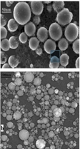
(1) Acidifying the base fluid, (2) adding lubricant and disperser, (3) using ultrasonic vibrations. The goal of all these techniques is to change the surface properties of a system and prevent settling in order to achieve a stable suspension. In the current study, 20–22nm Al2O3 nanoparticles were mixed with distilled water and stabilizers. It then continuously produces 100-watt ultrasonic pulses at 36 ± 3 kHz for 5 hours to break down the masses and accumulate nanoparticles by ultrasonic vibrator (Toshiba, India) before the agent is used in the fluid. The optimum volume concentration in this study was between 0.2 and 1. The pH of the fluids showed that the chemistry of the solutions was almost neutral. A new nanofluid was provided for each test and used immediately. The density of some nanofluid samples was measured before and after laboratory testing to check the stability of nanofluid emissions. No significant differences were observed in the measured density. The distribution of the main nanoparticles Al2O3 on a nanoscale can be observed by a transverse electron microscope (TEM) and SEM. Figure 1 (a) shows the SEM images of Al2O3 when the flow was set at 75 A.
Figure 1. (a) SEM image of Al2O3 particles (b) TEM image of particles Al2O3
The approximate size of the produced Al2O3 particle was measured directly from the SEM images by the Protec 2500 Optical Measurement System. In addition, the nanoparticles produced in Figure 1 are well rounded and uniform in size. Figure 1 (b) shows the TEM image of nanoparticle suspension. As shown in Figure 1 (b), the Al2O3 nanoparticles prepared by the proposed compound system, represent a good distribution of nanoparticles with an average size of 20–22nm. For this experiment, the relationship of the flow to the nanoparticles can be analyzed by different currents.
2.2 Investigation of pressure loss in piping systems based on ethylene glycol fluid
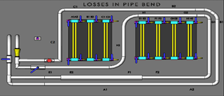
Power dissipation device from the piping system Resource can be seen in Figure 2.
Determining the flow pressure and flow in a pipe connection system (pipe network) is a general hydraulic issue. A pipe network is a system of pipes that consists of a single pipe or a complex system of pipes of different diameters and lengths. For example, the city's water supply network is a good example of a complex pipeline network. Typically, the network of pipes is designed in series, parallel, and circular in water supply systems. Therefore, it is necessary to measure the rate of energy loss in different places to perform accurate water supply calculations.
The network consists of two circuits (first and second circuits). The first circuit includes a Gate vatve No. 1, standard knee, 90° standard knee, straight pipes. The second circuit includes a ball valve No. 2 with a sudden opening, a sudden narrowing, 90° tee with different radiuses and straight pipes. Piezometer pipes are connected under pressure to measure the pressure loss in the components at the two ends of all components except for the valves.
Figure 2. Power dissipation device from the piping system Resource
The device has a water tank and a pump for water circulation in the piping system. The inlet water to the system is embedded on the device to measure the flow rate. The measurement unit of discharge is liters per minute.
Hand gauges have been used to measure pressure loss in both valve noses. All air bubbles must be removed from the pipes for testing. To this end, close valve 2 and open valve 1 to turn on the circuit after turning on the flow pump. Close the valve 1 and the flow control valve for a few minutes after the flow was set. Shake the piezometer hoses to direct the air bubbles trapped in different parts into the air-filled space above the piezometers. Close air vent valves (right valves) at the end of the manifold and return the discharge pump valve to a very low value so that the air inside the piezometers is ventilated. After this, close the discharge-regulating valve, turn off the pump, and allow the water level in the piezometers to loss to the desired value by slightly opening the upper and left valves of the piezometers. Then, first close the valve 1 and then the ventilation valve of the piezometers, so that the manometers of the first circuit are ventilated and ready for testing. Close valve 1 and open valve 2 and repeat the last steps to ventilate the second circuit.
2.3 Dimensional specifications of piping system
Some of the test information is:
Internal diameter of pipes: 16mm.
Internal diameter of the pipe after opening and before tightening: 26mm.
Internal diameter of the pipe after opening and before tightening: 16mm.
Distance between pressure gauges for straight pipes and bends: 1mm.
The curvature radius of knees:
G1/G2 knee: 2.5m.
J1/J2 knee: 5cm.
The continuity equation and Bernoulli Energy Relationships are used to calculate water flow in pipes with (1) and (2) relationships:
Continuity equation:
$\mathrm{Q}=\mathrm{A}_{1} \mathrm{~V}_{1}=\mathrm{A}_{2} \mathrm{~V}_{2}$ (1)
$\mathrm{Z} 1+\frac{P_{1}}{\rho g}+\frac{V_{1}^{2}}{2 g}=z_{2}+\frac{P_{2}}{\rho g}+\frac{V_{2}^{2}}{2 g}=h_{2}$ (2)
Figure 3. Loss due to sudden coefficient of friction
Pressure loss in pipes can be classified as follows:
A) A loss due to viscosity and internal friction of the fluid.
B) A loss caused by local complications or a sudden change in the cross-sectional area.
The loss in water flow pressure in a straight pipe with velocity V, length L, and constant diameter d is proportional to (3):
$\mathrm{h}_{1}=\mathrm{f} \frac{L}{d} \frac{V_{2}}{2 g}$ (3)
In the above equation, the Darcy-Weibach coefficient is the next base factor, which is a function of the Reynolds number and the surface roughness. One of the equations presented for calculating f in smooth pipes provided is Blasius, which is true for Re≤105:
$\mathrm{f}=\frac{0.3164}{R e^{025}}$ (4)
The f coefficient in the general condition of the pipes is determined by the moody diagram. The Reynolds number is also obtained from Eq. (5):
$\mathrm{Re}=\frac{v d}{u}$ (5)
:V=μ/ρ is systematic, which is equal in water at 25°C. The physical properties of water at different temperatures from 0°C to 100°C are available in the appendix of fluid mechanics books
The cross-section of the flow can suddenly increase or decrease. In pipefittings, the cross-sectional area changes abruptly due to the connection of two pipes with different concavities.
If low cross-section pipes are connected to high cross-section pipes, the localized loss due to sudden opening according is obtained from Eqns. (6) and (7). Loss due to sudden coefficient of friction can be seen in Figure 3.
$\mathrm{h}_{1}=\mathrm{k}_{\mathrm{e}} \frac{V_{1}^{2}}{2 g}=\frac{\left(V_{1}-V_{2}\right)^{2}}{2 g}$ (6)
$\mathrm{Ke}=\left[1-\left(\frac{\mathrm{d}_{1}}{\mathrm{~d}_{2}}\right)^{2}\right]^{2}$ (7)
In addition, if a pipe with a high cross-section is connected to a pipe with a lower cross-section, a local loss in the ratio (8) and (9).
$\mathrm{h}_{1}=\mathrm{k}_{\mathrm{e}} \frac{v_{2}^{2}}{2 g}=\frac{\left(\mathrm{V}_{1}-\mathrm{V}_{2}\right)^{2}}{2 g}$ (8)
$\mathrm{k}_{\mathrm{e}}=\left(\frac{A_{2}}{A_{1}}-1\right)^{2}=\left[\frac{1}{C_{c}}-1\right]^{2}$ (9)
Ac is the cross-sectional area at the accumulated area and Cc is the contraction coefficient. Approximate values of loss coefficient k for commercial parts in piping can be seen in Table 1.
The difference in balance between the two-piezometer pipes will give the size of the energy difference between the two sections. The value of the difference, or in other words, the measurement loss is displayed with hlw.
hlw=x-(Z2-Z1)=X+Z
Pressure loss can be calculated using these equations using the continuity equation and Bernoulli relations between points 1 and 2 and after simplification.
In the above relation, kc is the dimensionless coefficient of pressure loss in tightness and is obtained from the Table 2.
Local energy loss is caused by the turbulence of the water flow in the pipe knee. The value of this loss for curves is obtained from Eq. (10). Ka is the dimensionless coefficient that depends on the radius of the pipe and the angle of curvature.
$\mathrm{h}_{\mathrm{ln}}=\mathrm{k}_{\mathrm{a}} \frac{V^{2}}{2 g}$ (10)
One of the local connections is the valves, which cause a relatively large loss in flow due to the internal structure. The amount of energy loss in valves is obtained from Eq. (11).
$\mathrm{h}_{1}=\mathrm{k}_{\mathrm{a}} \frac{V^{2}}{2 . g}$ (11)
In the above equation, k1 is the energy coefficient in the valve, which is dimensionless and depends on the type of valve and the degree of its opening. If the valve is completely closed, k = ∞. Table 2 shows the approximate values of the energy coefficient of the valves and other connections.
Table 1. Approximate values of loss coefficient k for commercial parts in piping
|
Type of piece |
k-value |
|
|
Twisted |
Installed with flange |
|
|
Fully open Globe valve |
1 |
5 |
|
Gate valve |
0/2 |
0/1 |
|
Bent back |
1/5 |
0/2 |
|
Normal 90 reversible elbow |
1/5 |
0/3 |
|
90 reversible elbow with a lot of curvature |
0/7 |
0/2 |
|
Normal 45 reversible elbow |
0/4 |
- |
|
45 reversible elbow with a high curvature radius |
- |
0/2 |
Table 2. Pressure loss in tightness
|
A2/A1 |
0/0 |
0/1 |
0/2 |
0/3 |
0/4 |
0/6 |
0/8 |
1/0 |
|
K |
/500 |
/400 |
/400 |
/360 |
/300 |
/130 |
/060 |
/000 |
2.4 Obtaining the venture and orifice discharge coefficient
Changes in loss rate depending on current intensity for the components tested (venture meter, orifice, sudden opening, and 90-degree knee) then discharge measurement device can be seen in Figure 4.
Figure 4. Discharge measurement device
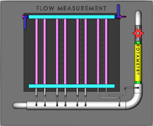
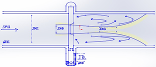
2.5 Device description
The discharge of the flow is measured by several types of flowmeters (venture meters, orifices, and rotameters) by this device. Moreover, the loss rate in flow meters, curves, and parts is measured where there is a sudden change in diameter (diffusion), so that the water flow is pumped into the system by the pump. First, the water enters a horizontal pipe after passing through the valve, which passes through a diffuser (sudden opening) after passing through the venture meter. Along the way, there is an orifice with a diameter of 20mm. After passing through the orifice, the flow enters a 90-degree knee, and finally it goes through a rotameter. The flow is measured by a rotameter. Manometers are used to measure static pressure along the way before and after the flowmeters, as well as before and after the diffuser and knee. The height of the water is measured by the dial behind the manometers.
The test components and their dimensions are as follows then components of flow discharge device can be seen in Figure 5:
1. venture meter with input diameter of 26mm and output diameter of 26mm and throat diameter of 16mm
2. Cone expansion from 26mm diameter to 50mm diameter.
3. Orifice meter with a diameter of 20mm
4. Knee 90 with a diameter of 56mm
5. Rotameter
Figure 5. Components of flow discharge device
The orifice is a usually round hole through which fluid flows and may have sharp edges or rounded edges. Installing a sharp edge orifice in the pipe causes it to shrink according to (Figure 6) jet passing through it.
Figure 6. Orifice in the pipe
For the incompressible flow, the Bernoulli equation is written between section 1 and section 2, i.e. the contracted section.
$\frac{V_{U}^{2}}{2 g}+\frac{p_{1}}{y}=\frac{V_{U}^{2}}{2 g}+\frac{p_{2}}{y}$ (12)
qin which, V2 is the theoretical value of contraction velocity. On the other hand, the equation of connection between two sections is expressed as follows:
$V_{2} \frac{\pi D_{1}^{2}}{4}=V_{2} D_{0} \frac{\pi D_{0}^{2}}{4}$ (13)
in which, C0=A2/A0 is the contraction coefficient. By removing V2 in the above equations:
$\frac{V_{21}^{2}}{2 g}\left[1-C_{1}^{2}\left(\frac{D_{0}}{D_{1}}\right)^{4}\right]=\frac{P_{1}-P_{2}}{Y}$ (14)
By solving the above equation, V2 is obtained as follows:
$V_{21}=\sqrt{\frac{2 g\left(P_{1}-P_{2}\right) / y}{1-C_{1}^{2}\left(D_{0} / D_{1}\right)^{4}}}$ (15)
If it is multiplied by C2, the actual velocity at the contraction is obtained:
$V_{21}=\sqrt{\frac{2\left(P_{1}-P_{2}\right) / p}{1-C_{1}^{2}\left(D_{0} / D_{1}\right)^{4}}}$ (16)
Finally, with the real speed hit on the jet level, the actual discharge is achieved:
$\mathrm{Q}=\mathrm{C}_{\mathrm{d}} \mathrm{A}_{0} \sqrt{\frac{2\left(P_{1}-P_{2}\right) / p}{1-C_{1}^{2}\left(D_{0} / D_{1}\right)^{4}}}$ (17)
in which, Cd =C1C2, is the orifice meter discharge coefficient.
The following equation can be used to calculate discharge in venture the help of Bernoulli's equation and by avoiding the loss of energy between the inlet sections in the venture condenser (Proving this equation is similar to proving an orifice relationship).
$\mathrm{Q}=\mathrm{C}_{\mathrm{d}} \mathrm{A}_{0} \sqrt{\frac{2\left(h_{1}-h_{2}\right)}{1-\left(D_{2} / D_{1}\right)^{4}}}$ (18)
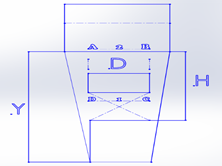
A rotameter is a vertical divergent tube in which there is a floating object. The specific gravity of a float is greater than that of a liquid. The fluid in the tube flows upwards and pushes the float upwards. The tube is clear and the float is visible. The pipe is calibrated, from which discharge is read directly.The equation gives calculates the discharge of incompressible flow passing through the venture tube due to the difference in monomeric height. The contraction coefficient is equal to one in venture tube. So, Cd =C1.
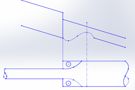
The difference in pressure and energy loss between the AB and D.C levels causes the cone to be immersed in equilibrium at altitude Y (Figure 3-7). If the energy loss is between (1) and (2) hH, according to Bernoulli's theorem:
$\frac{p_{1}}{y}=\frac{V_{1}^{2}}{2 g}+\frac{p_{2}}{y}+\frac{V_{2}^{2}}{2 g}+\mathrm{h}_{\mathrm{H}}+\mathrm{H}$ (19)
If the cross-sectional changes between (1) and (2) are ignored, the above equation V1+V2 can be written as follows:
$\frac{P_{1}-P_{2}}{Y}+H+h_{\mathrm{H}}$ (20)
Figure 7. Cross-sectional changes
Considering the balance of control volume of "ABCD":
$\mathrm{P}_{2} \mathrm{~A}_{2}+\mathrm{W}_{1}+\mathrm{W}_{\mathrm{W}}-\mathrm{P}_{1} \mathrm{~A}_{1}=0$ (21)
In which, W1 is the weight of the cone and WW is the weight of the water inside the control volume. By ignoring the changes in cross section A1= A2 and as a result:
$\left(\mathrm{P}_{1}-\mathrm{P}_{2}\right) \mathrm{A}=\mathrm{W}_{\mathrm{f}}+\mathrm{W}_{\mathrm{W}}$ (22)
After removing (P1 – P2) between the above equations hH = (Wf+ Ww) / YA1 –H, all values to the right of the equation are constant. As a result, hH will be constant for all y values. Given that this loss in energy depends on the rate of flow around the base of the cones. So, the flow rate in the conical base environment will also be constant. If this velocity is shown by V, then the flow intensity is:
$\mathrm{Q}=(\pi D d)^{V}$ (23)
In Figure 2, d = yθ. As a result:
$\mathrm{Q}=(\pi D d V)_{\mathrm{y}}$
The value in the rotameter is directly related to the height of the submerged cone (y).
Energy loss in flowmeters.
Localized lesions are caused by the following reasons:
Inlet or outlet of the pipe.
Sudden expansion or contraction.
The presence of knees, valves, etc.
Gradual expansion or contraction of the section.
In the orifice, the amount of energy loss is significant, and if it is ignored, a significant error in measurement occurs. In practice, the loss coefficient is used, which can be calculated for each of the devices using the following equation:
$\mathrm{K}=\frac{Q_{m}}{Q_{1}}$ (24)
in which, Q1 is the calculated discharge from the theatrical discharge and Qm is the actual calculated discharge. The value of K is generally a function of the shape and specifications of the device and the amount of discharge and fluidity of the fluid specifications.
The energy loss (h1) is obtained during a venture meter, orifice meter, or rotameter from the following equation.
$\mathrm{h}_{1}=\Delta \mathrm{H}=K^{V^{2}} / 2 g$ (25)
V is the speed at the input and deception of the device loss.
The loss factor (K) of each part can be obtained using the following equations by determining the loss in energy and kinetic energy of the input.
Loss in Venturi: ΔHAC = hA - hC.
Loss in Orifice: ΔHEF = hE - hF.
The loss in sudden expansion and according to Figure 8 expansion is considered from section 1 to section 2.
Figure 8. Loss in sudden expansion
The losses related to the diameter change in the above system are as follows:
$\mathrm{H}_{\mathrm{e}}=K_{e}^{V_{1}^{2}} / 2 g=\frac{\left(V_{1}-V_{2}\right)^{2}}{2 g}$ (26)
$\mathrm{~K}_{\mathrm{e}}=\left(1-\frac{A_{1}}{A_{2}}\right)^{2}=\left[1-\left(\frac{d_{1}}{d_{2}}\right)^{2}\right]^{2}$ (27)
The energy loss between points C and D is calculated from the following equation:
$\Delta \mathrm{H}_{\mathrm{CD}}\left(\mathrm{h}_{\mathrm{C}-} \mathrm{h}_{\mathrm{D}}\right)+\frac{V_{C}^{2}}{2 g}=\left(1-\frac{A_{1}}{A_{2}}\right)^{2}$ (28)
Knee energy loss can be obtained from the following equation with the help of Bernoulli Equation between the inlet and outlet of the knee as well as in the piezometric tubes.
$\Delta \mathrm{H}_{\mathrm{CD}}\left(\mathrm{h}_{\mathrm{C}^{-}} \mathrm{h}_{\mathrm{D}}\right)+\frac{V_{C}^{2}}{2 g}=\left(1-\frac{A_{G}}{A_{H}}\right)^{2}$ (29)
3.1 Test fluid: A mixture of ethylene glycol and water
3.1.1 Test method
The piezometers were described according to the method and were ventilated according to the device's instructions. Conduct the experiment in two modes (a) and (b) for the first and second circuit.
3.1.2 A-The first circuit
While valve 1 is completely open (circuit 1) and valve 2 is closed, complete the Table 3 for the different discharge rates and reviewing the pressure loss in circuit one and the fluid tested for water and ethylene glycol can be seen in Figure 9.
Figure 9. Reviewing the pressure loss in circuit one and the fluid tested for water and ethylene glycol
3.2 Analysis of the first circuit
The amount of volumetric discharge rate of the device in circuit number one is from 3L. s-1 to 18L.s-1. The measurement intervals of the discharges have a specific volume, time, and similar scale. As the flow rate increases, so does the pressure loss in circuit number 1. The lowest amount of pressure loss in direct pipes without changing the diameter of the connection angle is evident, and the highest rate of pressure loss is related to the points that have more knee angles with a sharper angle. The highest apparent pressure loss between different parts of the first circuit is in the certain range of 9L. s-1 (in discharge interval less than 10L.s-1) and in the range of 18L.s-1 (in discharge interval more than 10L.s-1). The loss in pressure at any point increases the pressure loss at different points, and evidence of this fact has been recorded and confirmed by piezometers from the beginning of the nanoscale flow in circuit number one to its end.
Second circuit: Close valve 1 and open valve 2 and complete the Table 4 for different flow rates and reviewing the pressure loss in circuit two and the fluid tested for water and ethylene glycol can be seen in Figure 10.
Figure 10. Reviewing the pressure loss in circuit two and the fluid tested for water and ethylene glycol
3.3 Second circuit analysis
The amount of volumetric discharge rate of the device in circuit number 1 s from 3L. s-1 to 18L.s-1. The measurement intervals of discharges have a specific volume, time, and similar scale. As the flow rate increases, the pressure loss in circuit number 1 also increases. The lowest rate of pressure loss in direct tubes with sudden opening is evident, and the highest rate of pressure loss is in areas with more knee angles.
The highest apparent pressure loss between different points of the second circuit is evident in the characteristic range of 9L. s-11 (in discharge interval less than 10L.s-1), in the knee points of E1/E2, and in the range of 18L.s-11 (in discharge interval more than 10L.s-1).
Table 3. Test fluid: A mixture of ethyleneglycol and water
|
Readings on piezometer tubes |
Duration (s) |
Input water volume (lit) |
Test number |
|||||
|
Elbow bend prop |
rectangular bend |
Right tube |
||||||
|
C2 |
C1 |
B2 |
B1 |
A2 |
A1 |
|||
|
5/44 44 41 5/37 37 37 |
5/48 55 5/62 79 86 86 |
51 50 5/49 5/45 43 42 |
55 62 5/68 5/86 5/93 97 |
50 5/51 5/53 55 5/55 5/55 |
53 59 65 79 83 5/85 |
LPM LPM LPM LPM LPM LPM |
3 6 9 12 15 18 |
Circuit 1 |
Table 4. Fluids tested for a mixture of ethylene glycol and water
|
Readings on piezometer tubes |
Duration (s) |
Input water volume v(lit) |
Test number |
|||||||
|
Bend 4 |
Bend 2 |
tightness |
openness |
|||||||
|
H2 |
H1 |
G2 |
G1 |
F2 |
F1 |
E2 |
E1 |
|||
|
5/35 37 5/37 5/38 5/38 39 |
48 52 61 5/45 72 76 |
47 47 46 5/44 5/42 5/41 |
5/50 5/56 5/67 75 5/83 5/89 |
5/40 5/41 5/45 5/47 49 50 |
42 5/46 57 5/63 5/71 76 |
42 44 47 48 48 5/48 |
44 51 5/61 69 5/77 5/82 |
l/m |
3 6 9 12 15 18 |
Circuit 2 |
The loss in pressure at any point increases the pressure loss at different points, and evidence of this fact has been recorded and confirmed by piezometers from the beginning of the nanoscale flow in circuit number one to its end. The most important factor in the highest rate of pressure loss is related to the knees due to the creation of vortex flows.
Equation and numerical analysis of the piping system using Bernoulli and volumetric discharge rate:
$\mathrm{Z}_{1}+\frac{P_{1}}{\rho g}+\frac{V_{1}^{2}}{2 g}=z_{2}+\frac{P_{2}}{\rho g}+\frac{V_{2}^{2}}{2 g}=h_{2}$
P_1≫P_2 Assumption
$V_{1} \ll V_{2}$
Z1=z_2
$\frac{P_{1}-P_{2}}{\rho g}=\frac{V_{2}^{2}-V_{1}^{2}}{2 g}$
$\Delta \mathrm{P} \propto \Delta \mathrm{V}$ (Pressure difference in manometers)
Q=AV (discharge of the device)
$A=\frac{\pi D^{2}}{4}$
All the mentioned equations can be solved in all steps by calculating the velocity. At each stage, the desired parameters can be calculated and analyzed, such as the coefficient of friction, Nusselt, Reynolds, the heat transfer coefficients, etc. data obtained from the test of a mixture of ethylene-glycol and aluminum nanocidal oxide fluid can be seen in Table 5 and obtained from the test of a mixture of ethylene-glycol and aluminum nanocidal oxide fluid can be seen in Table 6. The difference in pressure created by the Nano fluid of aluminum oxide can be seen in Figure 11.
Figure 11. The difference in pressure created by the nanofluid of aluminum oxide
3.4 General analysis of the circuit in terms of nanofluid use
Adding nanoparticles to metal nanoparticles in basic fluids such as ethylene glycol and water causes a significant increase in system pressure loss. The most important cause of this pressure loss is the vortex flow created at the end of the pipe path, especially in places where there are bending connections. Moreover, the points where the sudden change in the diameter of the pipe tends to decrease the diameter of the path. Local connections such as valves also exacerbate the nanoscale pressure loss. By using nanoparticles, the interaction and collision of particles and fluids is intensified and the discharge rate increases.
Table 5. Table of data obtained from the test of a mixture of ethylene-glycol and aluminum nanocidal oxide fluid
|
Liter/minute |
A1 |
A2 |
B1 |
B2 |
C1 |
C2 |
E1 |
E2 |
F1 |
F2 |
G1 |
G2 |
H1 |
H2 |
|
3 |
61 |
59 |
76 |
72 |
70 |
60 |
67 |
64 |
64 |
62 |
70 |
66 |
76 |
73 |
|
6 |
65 |
58 |
80 |
68 |
80 |
62 |
74 |
68 |
72 |
67 |
78 |
68 |
82 |
75 |
|
9 |
72 |
63 |
89 |
69 |
86 |
59 |
81 |
68 |
78 |
68 |
85 |
67 |
87 |
75 |
|
12 |
79 |
62 |
96 |
65 |
86 |
49 |
86 |
66 |
82 |
67 |
91 |
62 |
95 |
73 |
|
15 |
79 |
56 |
91 |
51 |
86 |
42 |
87 |
60 |
82 |
61 |
92 |
54 |
90 |
67 |
|
18 |
79 |
52 |
105 |
49 |
76 |
71 |
85 |
50 |
78 |
52 |
89 |
42 |
85 |
56 |
Table 6. Table of data obtained from the test of a mixture of ethylene-glycol and aluminum nanocidal oxide fluid
|
Lpm |
A1/A2 |
B1/B2 |
C1/C2 |
E1/E2 |
F1/F2 |
G1/G2 |
H1/H2 |
|
3 |
2 |
4 |
10 |
3 |
2 |
4 |
3 |
|
6 |
7 |
12 |
18 |
6 |
5 |
10 |
7 |
|
9 |
9 |
20 |
27 |
13 |
10 |
18 |
12 |
|
12 |
17 |
31 |
37 |
20 |
15 |
29 |
17 |
|
15 |
23 |
40 |
44 |
27 |
21 |
38 |
23 |
|
18 |
27 |
56 |
58 |
35 |
26 |
47 |
29 |
Table 7. The pressure loss caused by the flowmeter is mentioned in the measurement items
|
Flow rate (lpm) |
h1 (mm) |
h2 (mm) |
h3 (mm) |
h4 (mm) |
h5 (mm) |
h6 (mm) |
h7 (mm) |
h8 (mm) |
|
4 |
19 |
16 |
20 |
19 |
19 |
19 |
16 |
16 |
|
8 |
26 |
20 |
28 |
27 |
29 |
24 |
24 |
23 |
|
12 |
26 |
22 |
24 |
21 |
29 |
18 |
14 |
14 |
|
16 |
28 |
20 |
30 |
29 |
32 |
18 |
16 |
15 |
|
20 |
32 |
18 |
31 |
31 |
38 |
12 |
7 |
8 |
|
24 |
44 |
14 |
33 |
32 |
40 |
8 |
11 |
11 |
In various devices and systems, from open and closed, which are somehow related to fluid flow, it is generally necessary to measure the amount of fluid passing through a site. Measurement of water, oil, and gas flow in pipes with ducts can be considered as obvious examples. There are various ways to measure the intensity of fluid flow or discharge. Perhaps the simplest way to measure discharge is to measure the volume with the passing fluid flow over time. Flows are divided into two categories, portable flow meters, such as price flow meters, which are commonly used to measure the intensity of flow in rivers or channels and immovable flow meters installed in hydraulic facilities along the flow path; Such as overflows, water meters, venture meters, orifice meters, and rotameters. The pressure loss caused by the flowmeter is mentioned in the measurement items can be seen in Table 7 and the reviewing of the pressure loss of the device components with the base fluid can be seen in Figure 12.
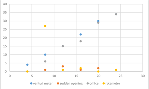
3.5 General analysis of pressure loss in flowmeter
Increasing the flow rate is the most important factor in the intensity of the pressure loss on each component. The results of changes in ventricular pressure loss and orifice are usually the same in a similar discharge. The most important factor is the sudden change in diameter and the phenomenon of rotation, which are associated with the greatest amount of energy loss. Changes in knee pressure loss and dilated area are much weaker than in other areas then the pressure loss table due to the flowmeter is mentioned in the measurement items can be seen in Table 8 and Figure 13.
Figure 12. Reviewing of the pressure loss of the device components with the base fluid
Figure 13. Reviewing the flow rate of different components of the flow rate
3.6 Analyzing the flow rate of the device components when using the base fluid
As the total discharge increases at each stage, the maximum discharge rate is in the path of the first equipment. Given the sudden change in the diameter (diffusion) of discharge located in the path of Venturi meter, it is slightly more than Orifice and this factor predicts an increase in further pressure loss in this area. Reviewing the pressure loss of the components of the flow meter with the base fluid can be seen in Figure 14 and 15.
Figure 14. Reviewing the pressure loss of the components of the flow meter with the base fluid
3.7 Analyzing the rate of pressure loss of the device components when using the base fluid
As can be seen from the results, the highest rate of pressure loss is felt in the venture meter equipment, especially in the sudden expansion of the diameter of the circuit. The pressure loss table due to the flowmeter in the measurement items mentioned according to the addition of titanium dioxide nanoparticles can be seen in Table 9 and Reviewing the pressure loss of the device components using Nano fluid can be seen in Figure 16.
Figure 15. Reviewing the pressure loss of the components of the flow meter with the base fluid
Figure 16. Reviewing the pressure loss of the device components using nanofluid
Table 8. Calculations of the pressure loss table due to the flowmeter is mentioned in the measurement items
|
The loss value in different parts |
|
|
|
|
|||
|
Elbow |
Orifice |
Sudden expansion |
venture |
Flow rate of Orifice |
Flow rate of venture |
Flow rate of Rotameter |
Flow rate of Rotameter |
|
4 8 12 16 20 24 |
3/00 5/22 8/14 10/24 13/92 19/24 |
1/101 1/02 2/04 2/28 2/73 3/01 |
0/0 1/21 2/00 2/12 2/23 2/92 |
0/002 0/02 0/012 0/021 0/028 1/080 |
0/0 0/001 0/001 0/002 0/001 0/01 |
0/0 0/02 0/001 0/014 0/020 0/030 |
0/0 0/0 0/002 0/002 0/0 0/0 |
Table 9. The pressure loss table due to the flowmeter in the measurement items mentioned according to the addition of titanium dioxide nanoparticles
|
Flow rate (lpm) |
h1 (mm) |
h2 (mm) |
h3 (mm) |
h4 (mm) |
h5 (mm) |
h6 (mm) |
h7 (mm) |
h8 (mm) |
|
4 |
21 |
17 |
20 |
20 |
18 |
18 |
17 |
17 |
|
8 |
37 |
27 |
35 |
36 |
35 |
29 |
27 |
27 |
|
12 |
29 |
14 |
25 |
28 |
29 |
14 |
13 |
14 |
|
16 |
36 |
14 |
30 |
31 |
32 |
14 |
17 |
15 |
|
20 |
38 |
8 |
30 |
32 |
33 |
4 |
8 |
8 |
|
24 |
45 |
11 |
37 |
38 |
40 |
6 |
10 |
11 |
3.8 Analysis of the flowmeter device in nanoscale conditions
As the component flow increases, the pressure loss of each component increases. Usually the results of changes in ventricular pressure loss and orifice in the same discharge are similar. The most important factor is the sudden change in diameter and the phenomenon of rotation, which are associated with the greatest amount of energy loss. Equation and numerical analysis of device specifications and proven formula:
(kg/s = Ẋ) Volumetric flow rate devices
Ẋ Mass flow. p = ṁ(m3/s)
Q=AV (discharge of the device)
$A=\frac{\pi D^{2}}{4}$
All the mentioned equations can be solved in all steps by calculating the velocity. At each stage, the desired parameters can be calculated and analyzed, such as the coefficient of friction, Nusselt, Reynolds, the heat transfer coefficients, etc. The data in the table above show the amount of pressure loss calculated in the flowmeter using the test fluid mixture and the addition of titanium dioxide nanoparticles.
The amount of changes made in different discharges at the output of each of the tested items indicates very little change in the flow meter.
In this test, the pressure loss of aluminum oxide nanoparticles and titanium dioxide in the base fluid of a mixture of ethylene glycol and water was tested as a fluid.
• The results of the experiments due to the addition of nanofluids to the mixture of water and ethylene glycol show the presence of nanoparticles in the test fluid have increased the pressure loss of nanofluid compared to the base fluid. This upward trend increases with increasing nanoparticle concentration. In fact, increasing the volume fraction of nanoparticles and reducing the temperature of the incoming fluid to the radiator are two factors that increase the viscosity of the nanofluid and increase its pressure loss.
• The results of the experiments for the two nanofluids indicate a higher-pressure loss and coefficient of friction of the nanofluid aluminum oxide than the nanofluid titanium dioxide. The reason for this can be expressed in the relatively high dimensions and density of aluminum oxide nanoparticles compared to 20nm titanium dioxide particles.
• The results of the experiment, due to the addition of titanium dioxide nanoparticles and aluminum oxide to the base fluid, indicate a slight difference in pressure loss in the pipelines, as well as the process of non-aggregation of nanoparticles in pipelines and non-correlation in tubular ducts for data obtained by adding titanium dioxide nanoparticles.
• The results show that the fluid tested was ethylene glycol and water in piping systems and closed circuits (such as radiators) to improve the heat transfer process.
|
P |
Pressure |
|
p |
Density |
|
V |
fluid velocity |
|
Z |
vertical distance of the point from the base line |
|
A |
Cross section |
|
h |
Energy loss |
|
L |
Length |
|
d |
Diameter |
|
C |
Contraction |
|
K |
Dimensionless |
|
H |
Head |
|
W |
Weight |
|
Q |
Discharge |
|
Re |
Reynolds number |
|
Subscripts |
|
|
c |
coefficient |
[1] Jamalei, E., Alayi, R., Kasaeian, A., Kasaeian, F., Ahmadi, M.H. (2018). Numerical and experimental study of a jet impinging with axial symmetry with a set of heat exchanger tubes. Mechanics & Industry, 19(1): 106. https://doi.org/10.1051/meca/2017017
[2] Adschiri, T., Yoko, A. (2018). Supercritical fluids for nanotechnology. The Journal of Supercritical Fluids, 134: 167-175. https://doi.org/10.1016/j.supflu.2017.12.033
[3] Kim, S., Song, H., Yu, K., Tserengombo, B., Choi, S.H., Chung, H., Kim, J., Jeong, H. (2018). Comparison of CFD simulations to experiment for heat transfer characteristics with aqueous Al2O3 nanofluid in heat exchanger tube. International Communications in Heat and Mass Transfer, 95: 123-131. https://doi.org/10.1016/j.icheatmasstransfer.2018.05.005
[4] Devendiran, D.K., Amirtham, V.A. (2016). A review on preparation, characterization, properties and applications of nanofluids. Renewable and Sustainable Energy Reviews, 60: 21-40. https://doi.org/10.1016/j.rser.2016.01.055
[5] Cabaleiro, D., Colla, L., Barison, S., Lugo, L., Fedele, L., Bobbo, S.J.N.R.L. (2017). Heat transfer capability of (ethylene glycol+ water)-based nanofluids containing graphene nanoplatelets: Design and thermophysical profile. Nanoscale Research Letters, 12(1): 1-11. https://doi.org/10.1186/s11671-016-1806-x
[6] Agromayor, R., Cabaleiro, D., Pardinas, A.A., Vallejo, J.P., Fernandez-Seara, J., Lugo, L. (2016). Heat transfer performance of functionalized graphene nanoplatelet aqueous nanofluids. Materials, 9(6): 455. https://doi.org/10.3390/ma9060455
[7] Sadri, R., Hosseini, M., Kazi, S.N., Bagheri, S., Zubir, N., Ahmadi, G., Dahari, M., Zaharinie, T. (2017). A novel, eco-friendly technique for covalent functionalization of graphene nanoplatelets and the potential of their nanofluids for heat transfer applications. Chemical Physics Letters, 675: 92-97. https://doi.org/10.1016/j.cplett.2017.02.077
[8] Pattanayak, B., Mund, A., Jayakumar, J.S., Parashar, K., Parashar, S. K. (2020). Estimation of Nusselt number and effectiveness of double-pipe heat exchanger with Al2O3–, CuO–, TiO2–, and ZnO–water based nanofluids. Heat Transfer, 49(4): 2228-2247. https://doi.org/10.1002/htj.21718
[9] Shakya, A., Yahya, S.M., Ansari, M.A., Khan, S.A. (2019). Role of 1-butanol on critical heat flux enhancement of TiO2, Al2O3 and CuO nanofluids. Journal of Nanofluids, 8(7): 1560-1565. https://doi.org/10.1166/jon.2019.1711
[10] Hussein, A.M., Kadirgama, K., Noor, M.M. (2017). Nanoparticles suspended in ethylene glycol thermal properties and applications: An overview. Renewable and Sustainable Energy Reviews, 69: 1324-1330. https://doi.org/10.1016/j.rser.2016.12.047
[11] Yang, L., Ji, W., Huang, J.N., Xu, G. (2019). An updated review on the influential parameters on thermal conductivity of nano-fluids. Journal of Molecular Liquids, 296: 111780. https://doi.org/10.1016/j.molliq.2019.111780
[12] Akhgar, A., Toghraie, D. (2018). An experimental study on the stability and thermal conductivity of water-ethylene glycol/TiO2-MWCNTs hybrid nanofluid: developing a new correlation. Powder Technology, 338: 806-818. https://doi.org/10.1016/j.powtec.2018.07.086
[13] Geng, Y., Khodadadi, H., Karimipour, A., Safaei, M.R., Nguyen, T.K. (2020). A comprehensive presentation on nanoparticles electrical conductivity of nanofluids: Statistical study concerned effects of temperature, nanoparticles type and solid volume concentration. Physica A: Statistical Mechanics and Its Applications, 542: 123432. https://doi.org/10.1016/j.physa.2019.123432
[14] Li, C.C., Hau, N.Y., Wang, Y., Soh, A.K., Feng, S.P. (2016). Temperature-dependent effect of percolation and Brownian motion on the thermal conductivity of TiO2–ethanol nanofluids. Physical Chemistry Chemical Physics, 18(22): 15363-15368. https://doi.org/10.1039/c6cp00500d
[15] Iacobazzi, F., Colangelo, G., Milanese, M., de Risi, A. (2019). Thermal conductivity difference between nanofluids and microfluids: Experimental data and theoretical analysis using mass difference scattering. Thermal Science, 23(6): 3797-3807. https://doi.org/10.2298/TSCI190404296I
[16] Mitra, D., Howli, P., Das, B.K., Das, N.S., Chattopadhyay, P., Chattopadhyay, K.K. (2020). Size and phase dependent thermal conductivity of TiO2-water nanofluid with theoretical insight. Journal of Molecular Liquids, 302: 112499. https://doi.org/10.1016/j.molliq.2020.112499
[17] Stalin, P.M.J., Arjunan, T.V., Matheswaran, M.M., Sadanandam, N. (2019). Experimental and theoretical investigation on the effects of lower concentration CeO2/water nanofluid in flat-plate solar collector. Journal of Thermal Analysis and Calorimetry, 135(1): 29-44. https://doi.org/10.1007/s10973-019-08670-2
[18] Kayabaşı, U., Kakaç, S., Aradag, S., Pramuanjaroenkij, A. (2019). Experimental investigation of thermal and hydraulic performance of a plate heat exchanger using nanofluids. Journal of Engineering Physics and Thermophysics, 92(3): 783-796. https://doi.org/10.1007/s10891-019-01987-7
[19] Khodabandeh, E., Rozati, S.A., Joshaghani, M., Akbari, O.A., Akbari, S., Toghraie, D. (2019). Thermal performance improvement in water nanofluid/GNP–SDBS in novel design of double-layer microchannel heat sink with sinusoidal cavities and rectangular ribs. Journal of Thermal Analysis and Calorimetry, 136(3): 1333-1345. https://doi.org/10.1007/s10973-018-7826-2
[20] Kayabaşı, U., Kakaç, S., Aradag, S., Pramuanjaroenkij, A. (2019). Experimental investigation of thermal and hydraulic performance of a plate heat exchanger using nanofluids. Journal of Engineering Physics and Thermophysics, 92(3): 783-796.
[21] Stephen, E.N., Asirvatham, L.G., Kandasamy, R., Solomon, B., Kondru, G.S. (2019). Heat transfer performance of a compact loop heat pipe with alumina and silver nanofluid. Journal of Thermal Analysis and Calorimetry, 136(1): 211-222. https://doi.org/10.1007/s10973-018-7739-0
[22] Akbari, A., Saidi, M.H. (2019). Experimental investigation of nanofluid stability on thermal performance and flow regimes in pulsating heat pipe. Journal of Thermal Analysis and Calorimetry, 135(3): 1835-1847. https://doi.org/10.1007/s10973-018-7388-3