Masoud Rahmani* | Amin Moslemi Petrudi | Mohammad Reza Pourdavood
© 2021 IIETA. This article is published by IIETA and is licensed under the CC BY 4.0 license (http://creativecommons.org/licenses/by/4.0/).
OPEN ACCESS
In this paper, the free and forced vibration of a functional rectangular plate in contact with a turbulent fluid is investigated. Functional plates have been considered due to their high thermal resistance to residual stresses. The geometry of the problem is that one side of the reservoir in which the fluid is placed is covered with a plate of Functionally Graded Material (FGM). In order to approximate the displacement of the plate, assuming the third-order theory of shear deformation, trigonometric harmonic test functions are used, which determine the boundary conditions of the simple and fixed plate support. In the equations governing fluid oscillating behavior, the potential velocity of the fluid is obtained by determining the boundary conditions of the fluid in the form of February series functions. To achieve the natural frequency of the plate in contact with turbulent fluid and the shape of the vibrating mode, the Rayleigh-Ritz energy method is used based on the minimum potential energy. In order to check the accuracy of the method used, the results of analytical solution after solving the equations by coding in Wolfram Mathematica software have been compared with numerical solution of Abaqus software and then with accurate results in references, which shows the appropriate accuracy of the solution. Finally, the effect of volumetric coefficient parameters, volume ratio, length ratio, plate thickness ratio, fluid height, reservoir width and boundary conditions on the natural frequency of the plate in contact with turbulent fluid has been investigated and analyzed.
free vibration, FGM, turbulent fluid, February series, Rayleigh-ritz method
FGM materials are a new type of composite material characterized by a gradual change in the microstructure and properties of the material. There are materials that have different properties in different areas due to the gradual change of chemical compounds, distribution and orientation or the size of the reinforcing phase in one or more dimensions. FGM materials are usually made of two materials, ceramic and metal. They are used in cases where the two sides of a piece are in completely different conditions, which requires metal properties on one side and ceramic properties on the other side. Among their manufacturing methods are powder metallurgy, vapor deposition method, Centrifugal Method, etc. Figure 1 shows how to change the properties from one side to the other side of the FGM.
Figure 1. Changing properties in FGM materials
These materials were first designed as thermal insulators for aerospace structures and nuclear reactors and are commonly used to extreme temperature changes. And the applications of these materials include cutting tools, furnaces, anti-heat coatings of turbine blades, etc. [1]. The use of FGM materials in engineering structures is increasing due to the high ability of these materials to control stress. In many of these applications, these materials are in contact with fluid, which necessitates the study of this type of loading in the behavior of structures shows FGM. The main advantages of FGM are as follows [2]: 1) When connecting two different materials, the gradient connection layer can eliminate the explicit interface and improve the interface Connection strength; 2) instead of the traditional uniform coating, reduce the structure of the thermal mismatch stress, improve the coating paste strength [3]. Functional gradient materials have been widely used in engineering structures, so it is particularly necessary to study their fracture properties. The FSI is a multifaceted problem in a system in which fluid flow leads to a change in solid structure and, on the other hand, a change in the solid form, leads to a change in the boundary conditions of the fluid problem. For instance, the airflow around the wing of the plane leads to change the shape of the wing (though partially), which will subsequently change the air flow pattern around the wings. Due to the many applications in the field of fluid coupling vibrations and structure, many studies have been done in this field. In 2004, Michler et al. [4] compared the discrete and continuous solving methods for numerical simulation of a fluid-structure interaction. The evaluation of the accuracy of these methods has shown that their cost and computational efficiency are also compared. In a discrete method at any time step, only a repetition of the fluid-structure interaction is required, resulting in a lower computational cost than the continuous method at any time step. In contrast to the discrete (component) method, it is a continuous method that appears to be uniquely stable and significantly more precise without any conditions. It can be used a larger time step than the discrete method for the same level with higher precision. But computations that take place in a continuous method at any time step are more expensive than discrete methods. However, for the continuous method, there is still potential for reducing computational costs. Chakrabarti in 2005 [5], in a book on numerical models of fluid-structure interaction, a wide range of numerical computing techniques have been introduced in the field of fluid mechanics and numerical calculations for the fluid effect on marine structures. In 2012, Hou et al. [6] In their study of numerical methods for fluid and structure interaction, the interaction between the incompressible fluid flow and the immersion structure, have been addressed in a nonlinear multi-physical phenomenon. The immersion method is an irregular mesh method. In the article, they examine the basic formulation of the immersion fringe method, immersion domain method and other immersion methods. Fluid-structure interaction in a turbine blade and it history studied by Tashakori et al. [7]. the fluid-structure interaction phenomenon and it history are studied by X and Y. they use simulation by using structural and fluid flow section of ANSYS software. The results show that by increasing the speed of inlet flow, the amount of blade tip deviation increases and also its impact increases on fluid pressure exerted on the rotor. Many studies have been conducted on the vibrations of FGM plates and plates in different modes and loads. Iqbal et al. [8] studied Vibration characteristics of FGM circular cylindrical shells filled with fluid using wave propagation approach. The fluid is considered non-viscous and incompressible. And the frequency for different modes is based on the end of the cylinder. Rahmani and Jafari [9] studied modal analysis of the fluid-structure interaction of a Rectangular Composite Plate. Using classical laminated plate theory, a closed form solution for natural frequencies of FSI is extracted. frequency response of plate-fluid system has been achieved for harmonic load. Tran et al. [10] studied Free vibration analysis of functionally graded doubly curved shell panels resting on elastic foundation in thermal environment. Burlayenko and Sadowski [11] studied Free vibrations and static analysis of functionally graded sandwich plates with three-dimensional finite elements. Nonlinear free vibration analysis of functionally graded plate resting on elastic foundation in thermal environment using higher-order shear deformation theory studied by Parida and Mohanty [12]. According to the mentioned background, the FSI vibrations of the thick FGM plates have not been analyzed analytically and usually numerical methods have been used. In the present paper, the vibrations of a relatively thick FGM plate are in contact with a turbulent fluid in a rigid reservoir whose frequencies and mods shape are presented and the effect of the geometric parameters of the plate and reservoir on frequency changes is investigated. In addition to free vibrations, forced vibrations under several different loads have also been investigated. The final solution of the equations and answer extraction has been done with Wolfram Mathematica 8 software.
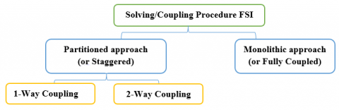
The FSI method used in this paper for numerical validation with Abaqus is a combination of CFD and CSM methods [13]. Generally solving problems with multiple physics is very difficult in analytical form. Therefore, such issues are often solved using numerical and experimental methods. Advanced numerical methods and popular commercial software applications in the CFD and CSM domains that make use of these methods, there are two different solutions for solving FSI problems using numerical software such as Abaqus, a Monolithic approach solution and Partitioned approach solving, which are described in each of these strategies. In Figure 2, you can see the breakdown of all types of FSI solutions [14].
Figure 2. Solving procedures in FSI [14]
In this study, partitioned approach and One-way coupling is used in Abaqus software, in this way, each of the problems is solved individually in the separate solvent, meaning that the fluid does not change during a structural solution, and vice versa. The fluid and structure equations are solved periodically in two solvents, and the information of each solution is exchanged at the point of contact of the fluid with the structure. You can see the process of this type of problem solving in Figure 3 The process of exchanging information at the level between the two ranges of solvers is called the solder coupler. It has two types of one-way couplings and two-way couplings.
Figure 3. Partitioned approach [15]
Figure 4. One-way coupling- flow chart [15]
One-way coupling is a mode that influences the movement of the fluid on the structure, But the structure's response to the fluid is ignored. As an example, in solving the issue of the propeller of the ship, the problem is considered as a one-way coupling. Figure 4 shows a graph of the one-way coupling method.
In solving the problem analytically, using the Wolfram Mathematica software, the equations of motion of the system are obtained in an integrated way. The equations of solid (structural) and fluid systems are solved simultaneously, and it is a monolithic solution method (Fully coupled).
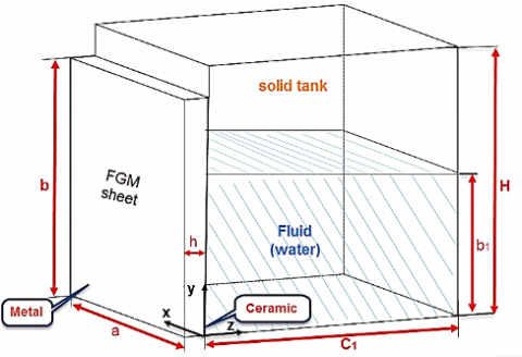
The issue under consideration is the vibrations of the FGM plate in contact with the Turbulent fluid. Figure 5 shows the general geometry and various parameters of the problem dimensions.
Figure 5. General geometry of the problem
In order to approximate the values of displacement from the boundary conditions, it has defined the functions that these functions must determine the boundary conditions, so they are defined as a double February series in the following form:
$u(x, y, t)=\sum_{n=1}^{N N} \sum_{m=1}^{M} a_{1} \sin \left(\frac{m \pi}{a} x\right) \cos \left(\frac{m \pi}{b} y\right)$
$v(x, y, t)=\sum_{n=1}^{N N} \sum_{m=1}^{M} a_{2} \sin \left(\frac{m \pi}{a} x\right) \cos \left(\frac{m \pi}{b} y\right)$
$w(x, y, t)=\sum_{n=1}^{N N} \sum_{m=1}^{M} a_{3} \sin \left(\frac{m \pi}{a} x\right) \sin \left(\frac{m \pi}{b} y\right)$
$(x, y, t)=\sum_{n=1}^{N N} \sum_{m=1}^{M} a_{3} \sin \left(\frac{m \pi}{a} x\right) \sin \left(\frac{m \pi}{b} y\right) \emptyset_{x}$
$(x, y, t)=\sum_{n=1}^{N N} \sum_{m=1}^{M} a_{3} \sin \left(\frac{m \pi}{a} x\right) \sin \left(\frac{m \pi}{b} y\right) \emptyset_{y}$ (1)
In these relations, t denotes time, and a6 a5 a4 a3 a2 a1 are functions whose value is obtained using the Rayleigh-Ritz method. M, NN are double displacement February series counters. Targeted rectangular plate length L, width a and thickness h are considered as Figure 4, which is made of a combination of ceramic and metal. Above the surface of the plate z=0 is a pure ceramic, and at the bottom of the surface of the plate z=-h is pure metal. All formulas here are assumed to be the elastic linear behavior of materials and small displacements and strains. The elastic properties of the material variable according to the thickness of the plates and the volume ratio according to the law. The properties of a point of width Z are as follows:
$V_{c}+V_{m}=1 . V_{m}=\left(\frac{-Z}{h}\right)^{\alpha}$
$E(z)=\left(E_{m}-E_{c}\right)\left(\frac{-Z}{h}\right)^{\alpha}+E_{c}$
$\rho(z)=\left(\rho_{m}-\rho_{c}\right)\left(\frac{-Z}{h}\right)^{\alpha}+\rho_{c}$ (2)
The rm is the metal density, rc is the ceramic density, Em is the metal Young's modulus, Ec is the ceramic Young's modulus, and Vm is the metal volume ratio and a is the exponent volume ratio. In this study, due to the study of thick plate of the third order theory, shear deformation has been used and in the program, the displacements of W, V, U in the direction, x, y, z are defined as follows:
$U(x . y . z . t)=z \emptyset_{x}(x . y . t)-\frac{4}{3 h^{2}} z^{3}\left(\emptyset_{x}+\frac{\partial w}{\partial x}\right)$
$V(x . y . z . t)=z \emptyset_{y}(x . y . t)-\frac{4}{3 h^{2}} z^{3}\left(\emptyset_{y}+\frac{\partial w}{\partial x}\right)$
$W(x . y . z . t)=w(x . y . t)$ (3)
In this relation, t indicates the time, fx, and fy of the deflection of the plate due to bending in the direction of the x, y, w axes, respectively and the displacement of the plate in the direction with the z axis. The relations between strain and displacement for this theory is as follows
$\varepsilon_{x x}=z \frac{\partial \emptyset_{x}}{\partial x}-\frac{4}{3 h^{2}} z^{3}\left(\frac{\partial \emptyset_{x}}{\partial x}+\frac{\partial^{2} w}{\partial x^{2}}\right) \rightarrow \varepsilon_{x x}=z k_{x}-\frac{4}{3 h^{2}} z^{3}\left(Q_{x}+K_{x}\right)$
$\varepsilon_{x y}=z\left(\frac{\partial \emptyset_{x}}{\partial y}+\frac{\partial \emptyset_{y}}{\partial x}\right)-\frac{4}{3 h^{2}} z^{3}\left(\frac{\partial \emptyset_{x}}{\partial y}+\frac{\partial \emptyset_{y}}{\partial x}+2 \frac{\partial^{2} w}{\partial x \partial y}\right)\rightarrow \varepsilon_{x y}=z k_{x}-\frac{4}{3 h^{2}} z^{3}\left(Q_{x y}+K_{x y}\right)$
$\varepsilon_{y y}=z \frac{\partial \emptyset_{y}}{\partial y}-\frac{4}{3 h^{2}} z^{3}\left(\frac{\partial \emptyset_{y}}{\partial y}+\frac{\partial^{2} w}{\partial y^{2}}\right) \rightarrow \varepsilon_{x x}=z k_{y}-\frac{4}{3 h^{2}} z^{3}\left(Q_{y}+K_{y}\right)$
$\begin{aligned} \varepsilon_{x z}=\frac{\partial w}{\partial x}+\emptyset_{x}-& \frac{4}{h^{2}} z^{2}\left(\frac{\partial w}{\partial x}+\emptyset_{x}\right) \rightarrow \varepsilon_{x z} \\ &=\left(1-\frac{4 z^{2}}{h^{2}}\right)\left(\emptyset_{x}+\frac{\partial w}{\partial x}\right) \end{aligned}$ (4)
k, xy values of the derivatives of the second order of transverse displacement of the plate are considered.
$Q_{x}=\frac{\partial^{2} w}{\partial x^{2}}, Q_{y}=\frac{\partial^{2} w}{\partial y^{2}}, Q_{x y}=2 \frac{\partial^{2} w}{\partial x \partial y}$
$R_{x}=\left(Q_{x}+\frac{\partial w}{\partial x}\right), R_{y}=\left(Q_{y}+\frac{\partial w}{\partial y}\right)$ (5)
According to Hooke's law, structural equations for FGM rectangular plates for third-order shear theory are shown below:
$\sigma_{x}=\frac{E(z)}{\left(1-v^{2}\right)}\left[\varepsilon_{x}+v \varepsilon_{y}\right]$
$\sigma_{y}=\frac{E(z)}{\left(1-v^{2}\right)}\left[\varepsilon_{y}+v \varepsilon_{x}\right]$
$\sigma_{x y}=\frac{E(z)}{2(1+v)} \varepsilon_{x y} \cdot \sigma_{x z}=\frac{E(z)}{2(1+v)} \varepsilon_{x z}$
$\sigma_{y z}=\frac{E(z)}{2(1+v)} \varepsilon_{y z}, \sigma_{z z}=0$ (6)
So, by placing Eq. (4) in Eq. (6), the following equations will be obtained.
$\begin{aligned} \sigma_{x}=& \frac{E(z)}{\left(1-v^{2}\right)}\left[\left[z k_{x}-\frac{4}{3 h^{2}} z^{3}\left(Q_{x}+K_{x}\right)\right]\right] +v\left[z k_{y}-\frac{4}{3 h^{2}} z^{3}\left(Q_{y}+K_{y}\right)\right] \end{aligned}$
$\begin{aligned} \sigma_{x}=& \frac{E(z)}{\left(1-v^{2}\right)}\left[\left[z k_{y}-\frac{4}{3 h^{2}} z^{3}\left(Q_{y}+K_{y}\right)\right]\right] +v\left[z k_{x}-\frac{4}{3 h^{2}} z^{3}\left(Q_{x}+K_{x}\right)\right] \end{aligned}$
$\sigma_{x}=\frac{E(z)}{2(1+v)}\left[z k_{x y}-\frac{4}{3 h^{2}} z^{3}\left(Q_{x y}+K_{x y}\right)\right]$
$\sigma_{x z}=\frac{E(z)}{2(1+v)}\left[\left(1-\frac{4 z^{2}}{h^{2}}\right) R_{x}\right]$
$\sigma_{y z}=\frac{E(z)}{2(1+v)}\left[\left(1-\frac{4 z^{2}}{h^{2}}\right) R_{y}\right]$ (7)
To obtain energy vibration equations, the potential and the target plate motion are required. The potential energy equation for the vibrating FGM rectangular plate of the following equation can be calculated:
$U_{p}=\frac{1}{2} \int_{0}^{a} \int_{0}^{b} \int_{-h}^{0}\left[\begin{array}{c}\sigma_{x x} \varepsilon_{x x}+\sigma_{y y} \varepsilon_{y y}+\sigma_{x y} \varepsilon_{x y} \\ +\sigma_{x z} \varepsilon_{x z}+\sigma_{y z} \varepsilon_{y z}\end{array}\right] d z d y d x$ (8)
The kinetic energy relation for FGM rectangular plate can also be calculated from the following relation:
$T_{P}=\frac{1}{2} \int_{0}^{a} \int_{0}^{b} \int_{-h}^{0} \rho(z)\left[\dot{U}^{2}+\dot{V}^{2}+\dot{W}^{2}\right] d z d y d x$ (9)
Fluid oscillation equations in contact with plates with assumptions: Non-viscous, non-compressible and non-rotating fluid with density rF, depth b1 and width rigid reservoir c1 are obtained according to Figure 4. The fluid velocity potential function is written using superposition principle as follows:
$\emptyset_{0}=\emptyset_{B}+\emptyset_{s}$ (10)
∅B is the fluid velocity potential due to plate vibration behavior and ∅S is the velocity potential due to turbulence fluid. Given that the fluid velocity potential must determine the Laplace equation, So:
$\nabla^{2} \emptyset_{0}=\nabla^{2} \emptyset_{B}+\nabla^{2} \emptyset_{s}=0$ (11)
The boundary conditions on the vertical and horizontal surfaces of the reservoir are as follows:
$\left.\frac{\partial \emptyset_{B}}{\partial x}\right|_{x=0}=0 .\left.\frac{\partial \emptyset_{B}}{\partial x}\right|_{x=a}=0$
$\left.\frac{\partial \emptyset_{B}}{\partial y}\right|_{y=0}=0 .\left.\frac{\partial \emptyset_{S}}{\partial x}\right|_{x=0}=0$
$\left.\frac{\partial \emptyset_{B}}{\partial z}\right|_{z=c_{1}}=0 .\left.\frac{\partial \emptyset_{S}}{\partial y}\right|_{y=0}=0$
$\left.\frac{\partial \emptyset_{S}}{\partial z}\right|_{z=c_{1}}=\left.0 \cdot \frac{\partial \emptyset_{S}}{\partial x}\right|_{x=a}=0$ (12)
For the free surface of the fluid, the boundary conditions without turbulence fluid will be as follows:
$\left.\emptyset_{B}\right|_{y=b 1}=0$ (13)
For boundary conditions elastic walls:
$\frac{\partial \emptyset_{B}}{\partial z}=\frac{\partial w(x \cdot y \cdot t)}{\partial t}$ (14)
Using the method of separating the variables and applying the boundary conditions, the answer of Eq. (10) of the fluid velocity potentials is calculated and written as follows in the code [16].
$\emptyset_{B}(x . y . z . t)=\sum_{l=0}^{\infty} \sum_{k=0}^{\infty} A_{l . k}(t) \cos \left(\frac{l \pi x}{a}\right) \cos \left(\frac{(2 k+1) \pi y}{2 b_{1}}\right)\times\left(e^{S_{1} z}+e^{S_{1}(2 c-z)}\right)$
$\emptyset_{S}(x . y \cdot z . t)=\sum_{i=0}^{\infty} \sum_{i=0}^{\infty} B_{i . j}(t) \cos \left(\frac{i \pi x}{a}\right) \cosh \left(S_{2} y\right) \cos \left(\frac{j \pi z}{c}\right)\quad(0 \leq x \leq a) \cdot\left(0 \leq y \leq b_{1}\right) \cdot\left(0 \leq z \leq C_{1}\right)$ (15)
In these relations $S_{1}=\pi \sqrt{(1 / a)^{2}+\left(\frac{2 k+1}{2 b_{1}}\right)^{2}} \quad' S_{2}=\pi \sqrt{(i / a)^{2}+\left(j / c_{1}\right)^{2}} \quad ' B_{i, j}$ the unknown constant is the velocity potential function due to turbulence fluid and Al.k(t) is the time constant of the velocity potential due to the oscillations of the plate and the following relation is obtained by applying the boundary condition of Eq. (14).
$A_{l \cdot k}(t)=\frac{\operatorname{cof} f_{1}}{a b_{1}} \int_{0}^{a} \int_{0}^{b_{1}} \dot{W}(x . y . t) \cos \left(\frac{l \pi x}{a}\right)\times \cos \left(\frac{(2 k+1) \pi y}{2 b_{1}}\right) d y d x /\left(S_{1}\left(1-e^{2 c S_{1}}\right)\right)$
$\begin{array}{rrr}1 \quad \text { if } l=k=0 \\\operatorname{cof} f_{1}=2 \text { if } l \text { or } k=0 \\4 \text { if land } k \neq 0\end{array}$ (16)
The fluid kinetic energy equations due to the vibration of the elastic plate and turbulence fluid according to the calculation of the fluid velocity potential are as follows [16]:
$T_{f_{B}}=\left.\frac{1}{2} \rho_{f} \int_{0}^{a} \int_{0}^{b_{1}} \emptyset_{B}\right|_{z=0}\left(-\frac{\partial w}{\partial t}\right) d y d x$
$T_{f_{S}}=\left.\frac{1}{2} \rho_{f} \int_{0}^{a b_{1}} \int_{0}^{\infty} \emptyset_{S}\right|_{z=0}\left(-\frac{\partial w}{\partial t}\right) d y d x$ (17)
The conditions of turbulence in the free surface of the fluid are as follows [17]:
$\left.\frac{\partial \emptyset_{0}}{\partial y}\right|_{y=b_{1}}=\left.\frac{\omega^{2}}{g} \emptyset_{s}\right|_{y=b_{1}}$ (18)
In this equation, w is the circular frequency of the coupling plate with the fluid and g is the acceleration of the Earth's gravity.
As a result, apply of Eq. (18) by (10):
$\left.\frac{\partial \emptyset_{B}}{\partial y}\right|_{y=b_{1}}+\left.\frac{\partial \emptyset_{S}}{\partial y}\right|_{y=b_{1}}=\left.\frac{\omega^{2}}{g} \emptyset_{S}\right|_{y=b_{1}}$ (19)
By multiplying the relation (19) in $\rho \mathrm{f} \emptyset_{S}$ and integrating on the free surface of the fluid:
$U_{\emptyset_{B}}+U_{\emptyset_{S}}=\omega^{2} T_{\emptyset_{S}}$ (20)
$\begin{aligned} U_{\emptyset_{B}}=& \rho F \int_{0}^{a} \int_{0}^{c}\left(\emptyset_{S} \frac{\partial \emptyset_{B}}{\partial y}\right)_{y=b_{1}} d z d x \\ T_{\emptyset_{S}} &=\frac{\rho F}{g} \int_{0}^{a} \int_{0}^{c}\left(\emptyset_{S}^{2}\right)_{y=b_{1}} d z d x \\ U_{\emptyset_{S}} &\left.=\rho F \int_{0}^{a^{c} c^{0}} \int_{0}^{\left(\emptyset_{S}\right.} \frac{\partial \emptyset_{S}}{\partial y}\right)_{y=b_{1}} d z d x \end{aligned}$ (21)
After calculating the values of energy and integrating in line with their thickness, now in this part of the code, the integration in the direction of x, y is done for all energy values. For this purpose, 3 integrals are defined by changing the variable and calling them energy values for each one, so that the complete energy values are finally integrated and ready to apply the Ritz method. In engineering application, the minimum principle of potential energy is used in order to obtain an approximate solution of problems whose exact solution is difficult or impossible. But in the Ritz method, the main problem is the correct guess to choose the correct displacement function because it leads to a lack of convergence or error in the answers. The conjectural functions must be in the boundary condition, and the Lagrangian function of the fluid plate system is as follows:
$\Pi=\sum U_{\max }-\sum T_{\max }$ (22)
Using the Ritz method, a special value equation of Eq. (22) is obtained:
$\frac{\partial \Pi}{\partial q_{m, n}}=0$ (23)
where, q the vector of generalized coordinates includes the coefficients of unknown time variables from the conjectural functions e.g.
$q=\left\{u_{m n} \cdot v_{m n} \cdot w_{m n} . \emptyset_{1_{m n}} . \emptyset_{2_{m n} } \cdot B_{i . j}\right\}$ (24)
After minimization, the equation is obtained as follows (Galerkin equation).
$\left(k_{p}+k_{R}\right) C_{m . n}-\omega^{2}\left[\begin{array}{c}\left(M_{P}+M_{f_{B}}\right) \\ C_{m . n}+M_{f s} B_{i, i}\end{array}\right]=0$ (25)
where:
$C_{m . n}=\left\{u_{m n} . v_{m n} \cdot w_{m n} . \emptyset_{1_{m n}} \cdot \emptyset_{2_{m n}}\right\}^{T}$ (26)
As a result, the Galerkin equation is obtained as follows [18]:
$\left[\begin{array}{cc}k_{P}+k_{R} & 0 \\ k_{\emptyset_{B}} & k_{\emptyset_{S}}\end{array}\right]\left\{\begin{array}{c}C_{m . n} \\ B_{i . j}\end{array}\right\}-\omega^{2}\left[\begin{array}{cc}M_{P}+M_{f_{B}} & M_{f_{S}} \\ 0 & M_{\emptyset_{S}}\end{array}\right]\left\{\begin{array}{c}C_{m . n} \\ B_{i . j}\end{array}\right\}=0$ (27)
where:
$k_{\emptyset_{S}}=\frac{\partial^{2} U_{\emptyset_{S}}}{\partial q_{i} \partial q_{j}} \cdot M_{\emptyset_{S}}=\frac{\partial^{2} T_{\emptyset_{S}}}{\partial q_{i} \partial q_{j}}\cdot$
$k_{\emptyset_{B}}=\frac{\partial^{2} U_{\emptyset_{B}}}{\partial q_{i} \partial q_{j}}$
$k_{P}=\frac{\partial^{2} U_{P}}{\partial q_{i} \partial q_{j}} \cdot k_{R}=\frac{\partial^{2} U_{R}}{\partial q_{i} \partial q_{j}}\cdot$
$M_{P}=\frac{\partial^{2} T_{P}}{\partial q_{i} \partial q_{j}}$
$M_{f B}=\frac{\partial^{2} T_{f B}}{\partial q_{i} \partial q_{j}} \cdot M_{f_{s}}=\frac{\partial^{2} T_{f S}}{\partial q_{i} \partial q_{i}}$ (28)
By placing a time function in the $W_{0}(x . y . t)=$ $\sum_{m=1}^{\infty} \sum_{n=1}^{\infty} W^{m n}(x . y) T^{m n}(t)$ relationship, the response of forced vibration to displacement the sheet is obtained as follows.
$W_{0}=\sum_{m=1}^{\infty} \sum_{n=1}^{\infty} \frac{W^{m n}(x \cdot y)}{K K \omega_{m n}} \int_{0}^{t} Q Q^{m n}(\tau) \operatorname{Sin}\left(\omega_{m n}(t\right. -\tau) d \tau$ (29)
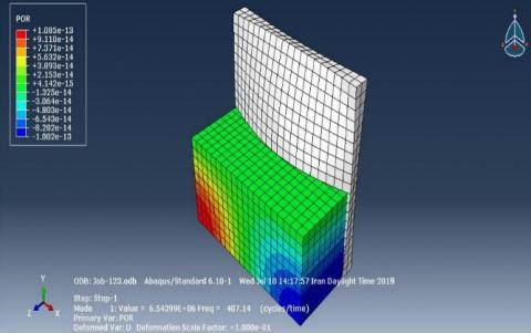
To evaluate, the results are compared with the numerical solution of Abaqus software and the results of previous research. Since the properties of FGM materials are not available in the library of numerical analysis software such as abacus, to define this type of material in the software, the sheet is cross-sectional divided into several parts. For each section, the mechanical properties associated with it are defined. However, the number of sections in the larger the cross section, the closer it is to the target material. In fact, in this study, the thickness of the sheet is divided into 64 sections. The element used to mesh the 3D element with 20 node, the size of the elements is 0.05m, and also the Structural mesh technique is used. Multilayer sheet modeling is shown in Figure 6.
Figure 6. Schematic of FGM sheet modeling in Abaqus software
Figure 7 shows a solution to the fluid and structure coupler problem in Abaqus.
The values obtained in this study have been validated with different sources and then the effect of sheet and fluid properties on the system frequency has been investigated. FGM rectangular sheet made of aluminum and ceramic, mechanical properties of these two materials are given in Table 1.
Figure 7. Schematic of FGM sheet modeling in contact with fluid in Abacus software
Table 1. FGM mechanical properties [8]
|
Material |
n |
E(GPa) |
$\rho$(Kg/m3) |
|
Al |
0.3 |
70 |
2702 |
|
Al2O3 |
0.3 |
380 |
3800 |
|
Ti-6Al-4V |
0.298 |
105.7 |
4429 |
|
Aluminum Oxide |
0.26 |
320.2 |
3750 |
Table 2 shows the values of the first 4 vibration frequencies for pure ceramic sheet and pure aluminum by analytical method using third-order shear deformation theorem and by numerical method using Abacus software. The results are compared with reputable sources. In this table, the simply supported boundary conditions, sheet length and width of 0.4 m and sheet thickness of 0.005 m are assumed.
Table 2. Comparison of the natural frequencies of a rectangular sheet with simply supported boundary conditions in terms of Hz
|
Mode number |
metal |
||
|
numerical |
ref [4] |
analytical |
|
|
1 |
114.90 |
143.67 |
144.96 |
|
2 |
361.96 |
360.64 |
360.64 |
|
3 |
361.96 |
360.64 |
360.64 |
|
4 |
577.89 |
575.87 |
575.87 |
|
Mode number |
ceramic |
||
|
numerical |
ref [4] |
analytical |
|
|
1 |
270.95 |
268.60 |
271.06 |
|
2 |
676.86 |
674.38 |
677.10 |
|
3 |
676.86 |
674.38 |
677.10 |
|
4 |
1080.70 |
1076.80 |
1082.48 |
Table 3. Comparison of dimensionless natural frequencies for FGM
|
Results |
$\alpha$ |
||||||
|
10 |
8 |
5 |
2 |
1 |
0.5 |
0 |
|
|
Reference [19] |
3.62 |
3.68 |
3.78 |
4.06 |
4.45 |
4.92 |
5.76 |
|
Reference [20] |
3.59 |
3.64 |
3.72 |
3.94 |
4.34 |
4.82 |
5.68 |
|
Present Work |
3.63 |
3.68 |
3.76 |
4.08 |
4.41 |
4.90 |
5.77 |
Now, the analytical results are then evaluated with other sources. In the Table 3 of natural frequencies without dimension $\beta=\left(\omega l^{2} / h\right) \sqrt{\frac{\rho_{c}}{E_{c}}}$ for FGM rectangular plates (Al/Al2O3) for simple boundary conditions with thickness to length ratio h/a=0.1 and the ratio of sides a/b=1 compared to references.
In the Table 4, the natural frequencies without dimension for the isotropic plate are in contact with the fluid for the values b1/b (The ratio of the height of the reservoir to the width of the plate) is obtained. Physical properties include $\mathrm{E}=25 \mathrm{Gpa}, \mathrm{v}=0.15$ and $\rho=2400 \mathrm{~kg} / \mathrm{m}^{3}$ considered and the geometric dimensions of the problem c1=100m, h=0.15m, b=a=10m and the boundary conditions are also a simple support.
Table 4. Comparison of natural non-dimensional isotropic plates
|
Results |
b1/b |
||||
|
1 |
0.8 |
0.4 |
0.3 |
0.2 |
|
|
Reference [21] |
1.036 |
1.173 |
2.196 |
2.451 |
3.064 |
|
Present Results |
0.860 |
1.031 |
2.190 |
2.401 |
3.019 |
After ensuring the accuracy of the results, the effect of different parameters on the frequency response of the problem is investigated below. Figure 8 shows a diagram of frequency changes in the first 10 vibration modes for this problem.
Figure 8. Frequency change in different modes
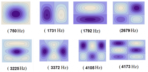
Figures 9 and 10 show the shape of the plate modes for the non-fluid state and the contact with the water fluid.
The base frequency changes of the plate are shown in the ratio of the sides and simple boundary conditions for the contact state of the plate with fluid and air in Figures 9 and 10. In this figure, the ratio of thickness to plate length α=0, h/a=0.1 and boundary conditions is simple. It has been observed that the natural frequencies of the plate in contact with the fluid are less than the plate in contact with air. Also, according to the results of these two shapes of the vibrating modes of the plate in contact with the fluid is distorted in relation to the plate in contact with the air. However, distortion in the shape of higher vibrational modes is more noticeable, which is due to the effect of fluid kinetic energies on the oscillations of the elastic plate.
Figure 9. The first eight modes of vibrating of FGM square plate for α=1 in air contact mode
Figure 10. The first eight modes of vibration of FGM square plate for a =1 in turbulent fluid contact state
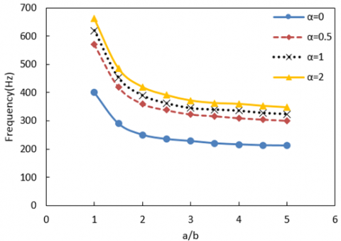
Figure 11. Plate base frequency changes in contact with the fluid relative to the sides
Figure 12. Plate base frequency changes in contact with the fluid relative to thickness
Figure 11 shows the frequency changes in the ratio of the sides of the plate in contact with the fluid for the coefficient of strength of different volumetric ratios and the ratio of thickness to the length of the plate is h/a=0.1 The length increases the width of the plate and the frequency of the vibration of the plate will decrease. Also, according to the figures, the higher the power law index, the higher the frequency of the system. As the volume ratio increases, the hardness of the plate increases and the percentage of ceramic in the plate increases. This is due to the direct relation between the frequency and the power law index (α).
Figure 12 shows the changes in the first frequency of the system relative to the thickness of the plate in contact with the fluid for the power law index (α). The Figure 12 shows that the higher the plate thickness ratio, the higher the vibrational frequency of the system. As the power law index increases, so does the frequency of the system. As the power law index increases, the hardness of the plate increases and the percentage of ceramic in the plate increases. This is the reason for the direct relation between the frequency and power law index.
Figure 13. The first frequency changes of the plate in contact with the fluid to the height
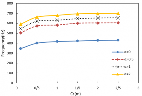
Figure 14. Plate base frequency changes in contact with fluid to reservoir width
Figure 13 shows the changes in the first four frequencies of the system to the height of the reservoir for different power law index. Due to the above figure, as the height of the reservoir increases, the amount of vibration frequency of the system decreases with a low slope. The ratio of the sides of plate a/b=1 and the ratio of thickness h/a=0.1 is assumed.
Figure 14 shows the changes in the base frequency of the system to the width of the reservoir. Depending on the figures, the higher the reservoir width, the higher the frequency of plate vibration. Then the curve gradually decreases and the slope reaches zero. As for the width of the large reservoirs, the frequency will not change with increasing width. Also, as the power factor of the volumetric ratio increases, so does the frequency of the system. As the volume ratio increases, the hardness of the plate increases, and the percentage of ceramic in the plate increases. This is due to the direct relationship between the frequency and power law index (α). The ratio of the sides of plate a/b=1 and the ratio of thickness h/a=0.1 is assumed.
Figure 15. Plate base frequency changes relative to the sides for the power factor of the power law index α=0
Figure 16. Plate base frequency changes relative to thickness for power law index α=0, and different boundary conditions
In Figures 15 and 16, the vibrational frequency changes for the fixed boundary conditions are similar to the simple boundary conditions. According to the results presented in these figures, due to the increase in hardness of the system due to the increase in geometric constraints at the plate boundaries for the same geometric and physical conditions, the natural frequency of the plate is simplified with the fixed boundary conditions.
In this section, to investigate the forced vibration in the time domain, the system's response to the harmonic, stepping, and triangular time distribution loads is obtained. According to the results obtained in the free vibration section, we now deal with the effect of volumetric coefficient parameters, sheet thickness ratio, fluid height and fluid tank width on the forced vibration response of the sheet-fluid system. The method used in this section is called the Eigenvalue Expansion method. In this section, the displacement curves of the central point of the rectangular FGM sheet (Al/Al2O3) have been checked. The boundary conditions are simply supported and a=b=1m.
The relationship of forces is as follows:
|
step force: |
$F(t)=\left\{\begin{array}{ll}1000 N & t \leq 0.01 \\ 0 & t>0.01\end{array}\right.$ |
|
trigonometric force: |
$\mathrm{F}(\mathrm{t})=1-\frac{\mathrm{t}}{0.05}, \mathrm{t} \leq 0.05$ (30) |
|
harmonic force: |
$\mathrm{F}(\mathrm{t})=1000 \operatorname{Sin}\left(\frac{\pi}{0.05} \mathrm{t}\right), \mathrm{t}>0$ |
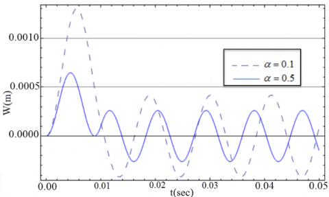
It is observed that according to Figure 17, the amplitude and period of the oscillations decrease with increasing the power factor of the power law index (α).
Figure 17. Changes in the response to the forced vibration of the FGM rectangular sheet to the power law index for the thickness ratio h / a=0.1 under the influence of the step force
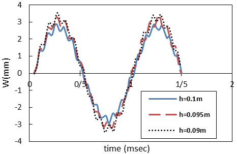
Figure 18. Changes in the response to forced vibration of the target rectangular sheet in proportion to the thickness for α=0 and under the influence of the triangular force
Figure 19. Changes in the response to forced vibration of the FGM rectangular sheet relative to the thickness for the effect of the harmonic force
Figure 20. Changes in the response to forced vibration of a FGM rectangular sheet in contact with a fluid for h/a=0.1 under the influence of a triangular force
In Figures 18 and 19, it can be seen from the curves that increasing the thickness reduces the amplitude of the oscillations and reduces the periodicity of the oscillations.
Figure 20 shows the changes in the vibration response of the target rectangular sheet in contact with the fluid with respect to the change in fluid height for α= 5, h / a=0.1 and c1=0.4m, which is affected by the triangular force. According to the figure, increasing the height of the fluid increases the amplitude of the oscillations and increases the periodicity of the oscillations.
Figure 21. Changes in the response to the forced vibration of a targeted rectangular sheet relative to the change in tank width for α=5 and h/a=0.1 b1=0.5 under the effect of a triangular force
The effect of the change in the width of the tank under the triangular force is shown in Figure 21.
According to Figure 21, increasing the width of the tank reduces the amplitude of the oscillations and also reduces the period of the oscillations.
In this study, the vibratory response of the FGM plate in contact with the turbulent fluid was investigated. The effect of volumetric coefficient parameters on volume ratio, length ratio, plate thickness ratio, fluid height, reservoir width and boundary conditions on the natural frequency of the plate in contact with turbulent fluid has been investigated and analyzed. The results show that first, as the width of the reservoir increases, the frequency of vibration of the plate will increase, then gradually the slope of the curve decreases and the slope reaches zero, so that for more width of the reservoir, the frequency will not change with increasing width. As the higher the reservoir height, the lower the vibration frequency of the system. When the ratio of length to width of the plate increases, the frequency of the vibration of the plate will decrease. According to the results, as the power factor of the volumetric ratio increases, so does the frequency of the system. As the volume ratio increases, the hardness of the plate increases and the percentage of ceramic in the plate increases. This is due to the direct relation between the frequency and the power law index (α). If the length-to-width ratio of the plate increases, the vibration frequency of the plate will decrease. In the next step, the forced vibration of the system is examined. The answer to the forced vibration of the FGM sheet is obtained in relation to the loads with harmonic, stepped and triangular time distribution.
[1] Azadi, M., Azadi, M. (2009). Nonlinear transient heat transfer and thermoelastic analysis of thick-walled FGM cylinder with temperature-dependent material properties using Hermitian transfinite element. Journal of Mechanical Science and Technology, 23(10): 2635. https://doi.org/10.1007/s12206-009-0716-6
[2] Kar, V.R., Panda, S.K., Tripathy, P., Jayakrishnan, K., Rajesh, M., Karakoti, A., Manikandan, M. (2019). Deformation characteristics of functionally graded composite panels using finite element approximation. In Modelling of Damage Processes in Biocomposites, Fibre-Reinforced Composites and Hybrid Composites, 211-229. https://doi.org/10.1016/B978-0-08-102289-4.00012-6
[3] Jin, Z.H., Feng, Y.Z. (2008). Thermal fracture resistance of a functionally graded coating with periodic edge cracks. Surface and Coatings Technology, 202(17): 4189-4197. https://doi.org/10.1016/j.surfcoat.2008.03.009
[4] Michler, C., Hulshoff, S.J., van Brummelen, E.H., de Borst, R. (2004). A monolithic approach to fluid-structure interaction. COMPUT FLUIDS, 33: 839-848. https://doi.org/10.1016/j.compfluid.2003.06.006
[5] Onate, E., Idelsohn, S.R., Celigueta, M.A., Rossi, R. (2008). Advances in the particle finite element method for the analysis of fluid–multibody interaction and bed erosion in free surface flows. Computer Methods in Applied Mechanics and Engineering, 197(19-20): 1777-1800. https://doi.org/10.1016/j.cma.2007.06.005
[6] Hou, G., Wang, J., Layton, A. (2012). Numerical methods for fluid-structure interaction—a review. Communications in Computational Physics, 12(2): 337-377. https://doi.org/10.4208/cicp.291210.290411s
[7] Tashakori, B.M., Elhami, M., Rabiee, A. (2016). Numerical analysis of fluid structure interaction phenomenon on a turbine blade. Fluid Mechanics and Aerodynamics Journal, 4(2): 1-11.
[8] Iqbal, Z., Naeem, M.N., Sultana, N., Arshad, S.H., Shah, A.G. (2009). Vibration characteristics of FGM circular cylindrical shells filled with fluid using wave propagation approach. Applied Mathematics and Mechanics, 30(11): 1393. https://doi.org/10.1007/s10483-009-1105-x
[9] Rahmanei, H., Jafari, A. (2016). Vibration analysis of a rectangular composite plate in contact with fluid. Iranian Journal of Mechanical Engineering Transactions of the ISME 17, 2: 67-83.
[10] Tran, Q.H., Duong, H.T., Tran, T.M. (2018). Free vibration analysis of functionally graded doubly curved shell panels resting on elastic foundation in thermal environment. International Journal of Advanced Structural Engineering, 10(3): 275-283. https://doi.org/10.1007/s40091-018-0197-x
[11] Burlayenko, V.N., Sadowski, T. (2020). Free vibrations and static analysis of functionally graded sandwich plates with three-dimensional finite elements. Meccanica, 55(4): 815-832. https://doi.org/10.1007/s11012-019-01001-7
[12] Parida, S., Mohanty, S.C. (2019). Nonlinear free vibration analysis of functionally graded plate resting on elastic foundation in thermal environment using higher-order shear deformation theory. Scientia Iranica. Transaction B, Mechanical Engineering, 26(2): 815-833.
[13] Biancolini, M.E. (2017). Fast Radial Basis Functions for Engineering Applications. Springer International Publishing.
[14] Olsson, S., Kesti, J. (2014). Fluid structure interaction analysis on the aerodynamic performance of underbody panels (Master's thesis). https://hdl.handle.net/20.500.12380/205833
[15] Bazilevs, Y., Calo, V.M., Hughes, T.J., Zhang, Y. (2008). Isogeometric fluid-structure interaction: theory, algorithms, and computations. Computational Mechanics, 43(1): 3-37. https://doi.org/10.1007/s00466-008-0315-x
[16] Xu, Y., Zhou, D. (2009). Three-dimensional elasticity solution of functionally graded rectangular plates with variable thickness. Composite Structures, 91(1): 56-65. https://doi.org/10.1016/j.compstruct.2009.04.031
[17] Abbasnia, A., Ghiasi, M. (2011). Estimation of three-dimensional base solution of turbulence with constant power and uniform velocity under boundary conditions of free surface and channel wall. 4th International Conference on Offshore Industries, 25: 202-210.
[18] Khorshid, K., Farhadi, S. (2013). Free vibration analysis of a laminated composite rectangular plate in contact with a bounded fluid. Composite Structures, 104: 176-186. https://doi.org/10.1016/j.compstruct.2013.04.005
[19] Hosseini-Hashemi, S., Taher, H.R.D., Akhavan, H., Omidi, M. (2010). Free vibration of functionally graded rectangular plates using first-order shear deformation plate theory. Applied Mathematical Modelling, 34(5): 1276-1291. https://doi.org/10.1016/j.apm.2009.08.008
[20] Zhao, X., Lee, Y.Y., Liew, K.M. (2009). Free vibration analysis of functionally graded plates using the element-free kp-Ritz method. Journal of sound and Vibration, 319(3-5): 918-939. https://doi.org/10.1016/j.jsv.2008.06.025
[21] Uğurlu, B., Kutlu, A., Ergin, A., Omurtag, M.H. (2008). Dynamics of a rectangular plate resting on an elastic foundation and partially in contact with a quiescent fluid. Journal of sound and Vibration, 317(1-2): 308-328. https://doi.org/10.1016/j.jsv.2008.03.022