Ancai Ma* | Sheliang Wang
© 2019 IIETA. This article is published by IIETA and is licensed under the CC BY 4.0 license (http://creativecommons.org/licenses/by/4.0/).
OPEN ACCESS
Under the action of earthquakes, the dynamic responses of cross-sea bridges are greatly influenced by the dynamic interaction between each pier and the surrounding water. Based on Morison equation, this paper mainly explores the responses of a continuous girder cross-sea bridge in uncontrolled and semi-active control modes, under the combined effect of earthquake and hydrodynamic pressure. First, a simplified two-degree-of-freedom (2DOF) analysis model was constructed for the bridge: the combined stiffness was proposed to reflect the effects of the bending and shear deformation features of the pier; the pier mass was aggregated on the top of the pier as the additional pier mass, using the shape function of linear deformation; the hydrodynamic pressure distributed on the pier was calculated by the Morison equation, converted into the equivalent node load on the top of the pier, and further transformed into the additional hydrodynamic mass. Then, a magnetorheological (MR) damper was added between the pier and the girder. The semi-active algorithm of the MR damper was designed based on the clipped-optimal control algorithm. The control force of the MR damper was optimized by the H2/LQG active control method. The results show that the hydrodynamic pressure changes the dynamic features of the bridge and increases the seismic responses of the bridge, calling for a stronger control force for semi-active control; the impact of hydrodynamic pressure must be considered in the seismic design of cross-sea bridges; the MR semi-active control can effectively suppress the dynamic responses of cross-sea bridges, enhancing the seismic safety of the bridge. The research results provide new insights into the vibration control of cross-sea bridges.
continuous girder bridge, hydrodynamic pressure, Morison equation, magnetorheological (MR) damper, semi-active control
Recent years has seen an unprecedented construction boom of cross-sea bridges in China. These bridges face a much more complex environment than the bridges over rivers and lakes. The piers of a cross-sea bridge are subject to the joint excitation of various loads induced by earthquake, wind and waves [1-3]. However, China has not yet acquired enough theoretical knowledge and empirical data about cross-sea bridges [4-6]. Therefore, it is of great engineering significance to develop a vibration control technique that suits cross-sea bridges.
Many vibration control devices and algorithms have emerged for engineering applications. The main control modes include passive mode, active mode, semi-active mode and hybrid mode. Among them, the semi-active control combines the merits of passive and active modes, and becomes a research hotspot in the field of control. However, few theories and test prototypes on semi-active control have been put into practice. The existing studies on semi-active control mainly tackle building structures [7-9]. There is little report on the semi-active control of bridge structures, not to mention cross-sea bridges. If applied to cross-sea bridges, semi-active control is expected to mitigate the damages caused by strong earthquakes and waves, and enhance the seismic safety of the bridges [10].
This paper proposes a simplified two-degree-of-freedom (2DOF) analysis model for a cross-sea bridge, calculates the dynamic pressure of a pier by Morison equation, and converts the result into the equivalent additional dynamic mass on the top of the pier. Then, a magnetorheological (MR) damper was added between the pier and the girder. The MR damper is a new-generation efficient semi-active controller, with advantages like simple structure, continuously adjustable damping force, fast response, large output, good durability, and minimal power consumption [11, 12]. The semi-active algorithm of the MR damper was designed based on the clipped-optimal control algorithm. The control force of the MR damper was optimized by the H2/LQG active control method. Finally, a control analysis program was prepared based on Matlab and Simulink, and used to simulate how the cross-sea bridge responses to the coupling effect of earthquake and hydrodynamic pressure, under semi-active control. The research results lay a theoretical basis for vibration control design of cross-sea bridges.
The remainder of this paper is organized as follows: Section 2 analyzes the structural motions based on Morison equation; Section 3 constructs the bridge dynamics analysis model; Section 4 models the motions of the controlled bridge structure; Section 5 presents the MR damper model and the semi-active control algorithm; Section 6 verifies the proposed control method through example analysis; Section 7 wraps up this research with several conclusions.
In the design of deep-water bridges, the hydrodynamic pressure can be computed by Morison equation, if the pier diameter is so small (pier diameter/wavelength<0.2) as to have little impact on wave motions. The equation assumes that the seawater is an ideal incompressible fluid with no vortex, and that the presence of the piers have no impact on wave motions. Under these assumptions, the speed and acceleration of the waves can be calculated by the wave theory according to the original wave scale [13, 14]. According to Morison equation, the force of water on the bridge structure mainly consists of inertial force and resistance, which respectively arises from the actions of the undisturbed acceleration and velocity fields along the direction of water movement. For a cylindrical structure with a small lateral size (i.e. a small diameter pier), the hydrodynamic pressure per unit length can be computed by:
$F=\rho \frac{\pi D^{2}}{4} \ddot{u}+C_{\mathrm{m}} \rho \frac{\pi D^{2}}{4}\left[\ddot{u}-\left(\ddot{x}_{\mathrm{g}}+\ddot{x}\right)\right]+\frac{1}{2} C_{\mathrm{d}} \rho D\left[u-\left(\dot{x}_{\mathrm{g}}+\dot{x}\right)\right] \dot{u}-\left(\dot{x}_{\mathrm{g}}+\dot{x}\right) |$ (1)
where, ρ is the water density; D is the length of the upstream face of the cylindrical structure; Ap is the area of the projection of the cylindrical structure in unit length perpendicular to the wave direction; $\dot{u}$ and $\ddot{u}$ are the speed and acceleration of the wave, respectively; $\dot{x}$ and $\ddot{x}$ are the relative speed and relative acceleration of the structure, respectively; $\dot{x}_{g}$ and $\ddot{x}_{g}$ are the speed and acceleration of ground motions, respectively; CM and CD are the coefficient of hydrodynamic inertia force and drag coefficient, respectively.
If the bridge is in still water, then $\dot{u}=\ddot{u}=0$, and formula (1) can be rewritten as:
$\begin{align} & F=-{{C}_{M}}\rho \frac{\pi {{D}^{2}}}{4}({{{\ddot{x}}}_{\text{g}}}+\ddot{x})- \\ & \frac{1}{2}{{C}_{D}}\rho {{A}_{p}}({{{\dot{x}}}_{\text{g}}}+\dot{x})\left| {{{\dot{x}}}_{\text{g}}}+\dot{x} \right| \\\end{align}$ (2)
where, the resistance term of the second term on the right side is nonlinear. Linearizing this term by the least squares (LS) method, the linearized Morison equation can be obtained as:
$\begin{align} & P=-\rho \left( {{C}_{M}}-1 \right)\frac{\pi }{4}{{D}^{2}}({{{\ddot{x}}}_{g}}+\ddot{x})- \\ & \frac{\rho }{2}{{C}_{D}}{{A}_{p}}\sqrt{\frac{8}{\pi }}({{{\ddot{x}}}_{g}}+\ddot{x}){{\sigma }_{{{{\ddot{x}}}_{g}}+\ddot{x}}} \\\end{align}$ (3)
The motions of the bridge structure under ground motions can be expressed as:
$\begin{align} & M\ddot{x}+C\dot{x}+Kx=-M{{{\ddot{x}}}_{\text{g}}}-{{C}_{M}}\rho \frac{\pi {{D}^{2}}}{4}({{{\ddot{x}}}_{\text{g}}}+\ddot{x})- \\ & \frac{1}{2}{{C}_{D}}\rho {{A}_{p}}({{{\dot{x}}}_{\text{g}}}+\dot{x})\left| {{{\dot{x}}}_{\text{g}}}+\dot{x} \right| \\\end{align}$ (4)
Compared with the inertia force, the hydrodynamic resistance is so small as to be negligible. Then, formula (4) can be rewritten as:
$M\ddot{x}+C\dot{x}+Kx=-M{{\ddot{x}}_{\text{g}}}-{{M}_{w}}({{\ddot{x}}_{\text{g}}}+\ddot{x})$ (5)
where, $M_{w}=\left(C_{M}-1\right) \rho \frac{\pi D^{2}}{4}$ is the additional hydrodynamic mass of the underwater structure. Next, formula (5) can be sorted out as:
$(M\text{+}{{M}_{w}})\ddot{x}+C\dot{x}+Kx=-(M+{{M}_{w}}){{\ddot{x}}_{\text{g}}}$ (6)
where, M, C and K are the matrices of structural mass, damping and stiffness, respectively.
As shown in formula (6), the structural impact of hydrodynamic pressure can be considered as the additional hydrodynamic mass that moves together with the structure. The coefficient of hydrodynamic inertia force CM depends on the shape of the structure. The CM value of a cylindrical pier is 2.
If a continuous girder bridge is highly regular, i.e. the adjacent piers/bearings have the same properties, the bridge can be simplified as a 2DOF model (Figure 1) with the main girder being a rigid body whose mass is concentrated on the bearings and each pier being an elastic body whose mass is concentrated on its top. The simplified 2DOF model can accurately display the dynamic response features of a regular continuous girder bridge under the action of earthquakes [15].
Figure 1. (a)-(c) Simplified 2DOF model and (d) placement of active and semi-active controllers
First, each pier was simplified as a one-degree-of-freedom (1DOF) cantilever system. If the pier is in a completely elastic state, the combined stiffness of the pier can be obtained based on the shear stiffness and bending stiffness:
$k_{1}=\frac{1}{H^{3} / 3 E I_{z}+H / A_{v} G}$ (7)
where, H is the height of the pier; Iz is the moment of inertia of the pier section; Av is the shear area of the pier; E is the elastic modulus; G is the shear modulus.
The pier deformation is assumed as linear to convert the mass distributed on the pier, $\bar{m}_{c}(x)$, into equivalent mass on the top of the pier. The pier deformation is assumed to obey the shape function:
$\psi(x)=\frac{1}{H} x$ (8)
If $\bar{m}_{c}(x)$ is known, the mass distributed on the pier can be aggregated on the top of the pier, forming the additional mass of the pier:
$m^{*}=\int_{0}^{H} \bar{m}_{c}(x) \psi^{2}(x) d x$ (9)
Substituting the shape function (8) into (9), we have:
$m^{*}=\int_{0}^{H} \bar{m}_{c}(x)\left(\frac{x}{H}\right)^{2} d x=\frac{\bar{m}_{c} H}{3}$ (10)
The hydrodynamic pressure acts on the pier in the form of distributed load. According to the principle of static equivalence, the distributed hydrodynamic pressure on the pier unit can be converted into the equivalent node load on the top of the pier by [16]:
$\left\{\begin{array}{l}{\mathrm{f}_{e i}=\frac{\bar{m}_{w}(x) h}{2}\left(2-2 \frac{h^{2}}{H^{2}}+\frac{h^{3}}{H^{3}}\right)} \\ {\mathrm{f}_{e j}=\bar{m}_{w}(x) h-\mathrm{f}_{e i}}\end{array}\right.$ (11)
where, fei and fej are the equivalent node load on the bottom and the top of the pier, respectively; $\bar{m}_{w}(x)$ is the hydrodynamic pressure distributed along the height of the pier.
The equivalent node load on the top of the pier was further transformed into the additional hydrodynamic mass on the top of the pier, to facilitate the use of the equation about structural motions, which is developed based on the Morison equation.
Under the presence of controller and seismic excitation, the motions of the bridge structure can be expressed as:
$\left\{\begin{array}{l}{\mathbf{M} \ddot{\mathbf{X}}(t)+\mathbf{C} \dot{\mathbf{X}}(t)+\mathbf{K} \mathbf{X}(t)=\mathbf{B}_{s} u(t)+\mathbf{M} \mathbf{r} \ddot{x}_{g}(t)} \\ {\mathbf{X}\left(t_{0}\right)=\mathbf{X}_{0}, \quad \dot{\mathbf{X}}\left(t_{0}\right)=\dot{\mathbf{X}}_{0}}\end{array}\right.$ (12)
where M, C and K are the matrices of structural mass, damping and stiffness, respectively; $\boldsymbol{X}(t)$ and $\dot{\boldsymbol{X}}(t)$ the displacement and velocity vectors of the structure relative to the ground, respectively; Bs is the position matrix of the controller; u(t) is the control force vector; r is the position vector of seismic excitation; $\ddot{x}_{g}(t)$ is the seismic excitation; $\boldsymbol{X}\left(t_{0}\right)$ and $\dot{\boldsymbol{X}}\left(t_{0}\right)$ are the initial displacement and speed of the structure, respectively.
To facilitate the implementation of the control system, the structural motion Eq. (12) can be illustrated in the form of state space:
$\dot{\mathbf{Z}}(t)=\mathbf{A} \mathbf{Z}(t)+\mathbf{B} u(t)+\mathbf{E} \ddot{x}_{g}(t)$ (13)
where, Z(t) is the state vector; A is the system matrix; B is the position indication matrix of the controller; E is the seismic action vector. These vectors and matrices can be expressed as:
$\mathbf{Z}=\left\{\begin{array}{l}{\mathbf{X}} \\ {\mathbf{X}}\end{array}\right\}, \mathbf{A}=\left[\begin{array}{cc}{\mathbf{0}} & {\mathbf{I}} \\ {\mathbf{- M}^{-1} \mathbf{K}} & {\mathbf{- M}^{-1} \mathbf{C}}\end{array}\right]$
$\mathbf{B}=\left[\begin{array}{c}{\mathbf{0}} \\ {\mathbf{M}^{-1} \mathbf{B}_{s}}\end{array}\right], \mathbf{E}=\left\{\begin{array}{l}{\mathbf{0}} \\ {\mathbf{- r}}\end{array}\right\}$ (14)
For the 2DOF model, there exist:
$\mathbf{M}_{0}=\left[\begin{array}{cc}{m_{1}} & {0} \\ {0} & {m_{2}}\end{array}\right], \mathbf{M}_{w}=\left[\begin{array}{cc}{m_{w}} & {0} \\ {0} & {0}\end{array}\right]$
$\mathbf{K}=\left[\begin{array}{cc}{k_{1}+k_{2}} & {-k_{2}} \\ {-k_{2}} & {k_{2}}\end{array}\right], \mathbf{B}_{\mathrm{S}}=\left[\begin{array}{c}{-1} \\ {1}\end{array}\right], \mathbf{X}=\left\{\begin{array}{l}{x_{1}} \\ {x_{2}}\end{array}\right\}$ (15)
where, $m_{1}=m^{*}$ is the additional mass on the top of the pier; $m_{2}$ is the mass aggregated to the upper part of the bridge; $m_{w}$ is the additional hydrodynamic mass converted to the top of the pier; $k_{1}$ and $k_{2}$ are the combined stiffness of the pier and the equivalent stiffness of the bearing, respectively. Note that $M=M_{0}+M_{w}$ if $m_{w}$ is considered, and $M=M_{0}$ if otherwise. The damping matrix of the structure can be determined by the damping ratios of the first two order modes according to Rayleigh damping.
5.1 MR damper model
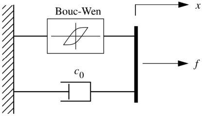
The MR damper selected for this research is a shear damper based on parallel plates. Here, the damper is simulated by the phenomenological model proposed by Dyke et al. [17] (Figure 2).
Figure 2. Model of the MR damper
The control force fs provided by the MR can be expressed as [18]:
$f_{s}(t)=c_{0} \dot{x}(t)+\alpha z(t)$ (16)
$\dot{z}=-\gamma|\dot{x}| z|z|^{n-1}-\beta \dot{x}|z|^{n}+A \dot{x}$ (17)
where, $\dot{x}$ is the relative speed across the two ends of the damper; $z$ is the hysteresis variable based on the Bouc-Wen model. By adjusting the values of $\gamma, \beta, n$ and $A,$ it is possible to control the following two properties of the hysteresis curve of the MR damper in the loading/unloading phase; the linear features, and the smoothness of the transition segment through the yielding. The correlation of model parameters $c_{0}$ and $\alpha$ with the input voltage $u_{c}$ can be expressed as:
$c_{0}=c_{0 a}+c_{0 b} u_{c} ; \alpha=\alpha_{a}+\alpha_{b} u_{c}$ (18)
The resistance inside the MR damper has a dynamic effect on the bridge structure. The dynamic features of the damper under an applied voltage can be eliminated by a first-order delay. Thus, the input voltage uc should be processed into the actual input voltage of the MR damper by the following first-order delay filter:
$\dot{u}_{c}=-\eta_{s}\left(u_{c}-u_{a}\right) \operatorname{trace}_{u, P, S, N} r_{2}$ (19)
where, $u_{i}=G_{i} z=G_{p i} x+G_{d i} \dot{x}=a_{p} G_{p i} x+a_{d} G_{d i} \dot{x} \quad$ is an indicator of the response time of the damper (the greater the $G_{p i}$ value, the shorter the response time); $u_{a}$ the actual voltage of the control loop.
5.2 The semi-active control algorithm of the MR damper
During semi-active control, the voltage applied to the MR damper varies with time, and depends on the selected control algorithm. In this paper, the clipped-optimal control algorithm is selected to realize semi-active control [19]. The algorithm computes the theoretical control force fc based on an active controller Kc, the observed structural response xm and the measured MR control force fm:
$f_{\mathrm{c}}=L^{-1}\left\{-K_{\mathrm{c}}(s) L\left\{\begin{array}{c}{x_{m}} \\ {f_{m}}\end{array}\right\}\right\}$ (20)
where, $L(\cdot)$ is the Laplace transform operator.
Since the damping force provided by the MR depends on the applied voltage and the relative speed across the MR damper, the theoretical control force fc can be tracked by adjusting the MR control force through regulation of the input voltage. To minimize the gap between the MR control force and the theoretical control force, the voltage applied to the MR can be computed by:
$v_{i}(t)=V_{c i}(t) H\left(\left\{f_{c i}(t)-f_{m i}(t)\right\} f_{m i}(t)\right)$ (21)
$V_{c i}=\left\{\begin{array}{ll}{\mu_{i} f_{c i},} & {f_{c i} \leqslant f_{\max }} \\ {V_{\max },} & {f_{c i}>f_{\max }}\end{array}\right.$ (22)
where, $f_{\text {max }}$ is the maximum output of the MR damper; $V_{\text {max is }}$ the maximum voltage applied to the MR damper; $f_{c i}$ is the control force obtained by the control algorithm; $\mu_{i}$ is the gain from voltage-to force-conversion; $V_{c i}$ is the control voltage; $H(\cdot)$ is the Heaviside step function.
In theory, any active control algorithm can be used to design the optimal controller Kc, which offers the theoretical control force. This paper selects the most successful engineering control method, H2/LQG, to design the main controller for the semi-active control of the MR damper. Th control output and observation output of the system can be respectively expressed as:
$Y_{z}(t)=C_{z} X(t)+D_{z} u(t)+F_{z} \ddot{x}_{g}(t)$ (23)
$Y_{m}(t)=C_{m} X(t)+D_{m} u(t)+F_{m} \ddot{x}_{g}(t)$ (24)
It is assumed that the system noise and measurement noise are both zero-mean Gaussian white noises. Then, the covariance matrices of the two types of noises can be determined by the third-generation benchmark model: both covariance matrices are diagonal matrices; the diagonal element of the covariance matrix of system noise and that of measurement noise were set to 25 and 1, respectively. On this basis, the quadratic objective function of H2/LQG control can be expressed as:
$J=\lim _{\tau \rightarrow \infty} \frac{1}{\tau} \mathrm{E}\left[\int_{0}^{\tau}\left\{\left(C_{z} x+D_{z} u\right)^{\mathrm{T}} Q\left(C_{z} x+D_{z} u\right)+R u^{2}\right\} d t\right]$ (25)
where, R and Q are the weight matrices that balance the structural response and the control force:
$Q=\left[\begin{array}{cc}{q_{d} I} & {0} \\ {0} & {q_{a} I}\end{array}\right], R=\beta I$ (26)
where, $q_{d}$ and $q_{a}$ are the displacement weight and acceleration weight of the pier top and main girder, respectively; $\beta$ is the weight of the control force.
According to the separation principle, the controller design and state estimation were processed separately. First, the optimal control law can be determined based on the linear quadratic optimal control theory:
$u=-K_{u} \hat{x}$ (27)
where, $\hat{x}$ is the system state vector estimated by the Kalman filter; $K_{u}$ is the full state feedback gain matrix.
In general, the optimal state estimation by the Kalman filter can be expressed as:
$\dot{\hat{x}}=A \hat{x}+B u+L\left(y_{\mathrm{m}}-C_{\mathrm{m}} x-D_{\mathrm{m}} u\right)$ (28)
where, L is the observation gain matrix of the stable Kalman filter.
To facilitate computer implementation, the controller can be converted into a compensator in the form of the following state equations through linear transform [18]:
$\left\{\begin{array}{l}{x_{k+1}^{c}=A_{c} x_{k}^{c}+B_{c} y_{k}} \\ {u_{k}=C_{c} x_{k}^{c}+D_{c} y_{k}}\end{array}\right.$ (29)
where, $A_{c}=A-B K_{u}-L C_{m}+L D_{m} K_{u}$; $B_{c}=L$; $C_{c}=-K_{u}$; $D_{c}=0$; $y_{k}=\left[\begin{array}{ll}{y_{m}} & {f_{m}}\end{array}\right]^{\mathrm{T}}$.
The proposed model was applied to analyze the seismic response and control of a continuous girder cross-sea bridge. The bridge has several cylindrical solid piers (diameter: d- $3.0 \mathrm{m} ;$ height: $\mathrm{H}=28.2 \mathrm{m}$ ) and the water depth $\mathrm{h}=20 \mathrm{m}$. Half of the mass of the two spans adjacent to a pier was taken $\mathrm{m}_{2}=500,000 \mathrm{kg},$ and aggregated on the bearing. The elastic was computed as $1.587 \times 10^{7} \mathrm{N} / \mathrm{m}$. The equivalent mass on the top of the pier is $166,112 \mathrm{kg}$. The equivalent stiffness of the bearing is $7.69 \times 10^{6} \mathrm{N} / \mathrm{m}$. The damping ratios were all set to $0.05 .$ Then, an MR damper (maximum rated output: $1,000 \mathrm{kN}$; maximum working voltage: $10 \mathrm{V} ;$ power: $50 \mathrm{W}$ ) was installed between the pier top and the girder. The corresponding parameters of the mechanical model include: $\alpha_{a}=1.0782 \times 10^{5}\mathrm{N} / \mathrm{cm}$, $\alpha_{b}=4.9616 \times 10^{5} \mathrm{N} /(\mathrm{cm} \cdot \mathrm{V})$, $c_{0 a}=4.40 \mathrm{Ns} / \mathrm{cm}$, $c_{0 b}=44.0$$\mathrm{Ns} /(\mathrm{cm} \cdot \mathrm{V})$, $n=1$, $A=1.2$, $\gamma=3 \mathrm{cm}^{-1}$ and $\eta_{s}=50 \mathrm{s}^{-1}$.
Without loss of generality, the seismic excitation was simulated with four common ground motions in benchmark problems, namely, El Centro wave (NS, 1940), Hachinohe wave (NS, 1968), JMA Kobe wave (NS, 1995) and Northridge wave (NS, 1994) [20-21]. The dominant frequencies are 1.47 Hz, 0.36 Hz, 1.46 Hz and 0.63Hz, respectively, and the maximum acceleration peaks are 3.417 m/s2, 2.250 m/s2, 8.178 m/s2 and 8.268m/s, respectively. The target bridge is designed to withstand a magnitude 8 earthquake. The amplitude of the input seismic wave was adjusted at the step length of the peak ground acceleration (PGA) of 0.2g.
Next, a program was prepared based on Matlab and Simulink, and used to simulate how the cross-sea bridge responses to the coupling effect of earthquake and hydrodynamic pressure, under semi-active control.
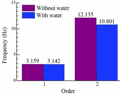
Figure 3 compares the first- and second-order frequencies of the bridge structure with and without water. It can be seen that the vibration frequency of the structure decreased after the addition of water, indicating that the presence of water changes the dynamic features of the structure.
Figure 3. Comparison of first- and second-order frequencies
To disclose the effect of hydrodynamic pressure on the seismic response of the bridge, the seismic responses were computed under the presence (with water) and absence (without water) of hydrodynamic pressure, respectively. Some of the calculated results are listed in Table 1, which presents the horizontal pier-top displacement, bearing deformation and the maximize control force of MR semi-active control. Figure 4 shows the time histories of the pier-top horizontal displacement and bearing deformation under the action of El Centro wave.
Table 1. Comparison of seismic responses in with water and without water conditions
|
Uncontrolled pier-top displacement/cm |
Uncontrolled bearing deformation/cm |
Maximum semi-active control force/kN |
|||||||
|
With water |
Without water |
Change rate (%) |
With water |
Without water |
Change rate (%) |
With water |
Without water |
Change rate (%) |
|
|
El Centro |
4.39 |
4.25 |
-3.2 |
7.51 |
7.92 |
5.5 |
320 |
321 |
0.3 |
|
Hachinohe |
6.33 |
6.85 |
8.2 |
11.31 |
11.26 |
-0.4 |
569 |
589 |
3.5 |
|
JMA Kobe |
3.64 |
3.95 |
8.5 |
6.76 |
7.09 |
4.9 |
321 |
327 |
1.9 |
|
Northridge |
6.55 |
6.36 |
-2.9 |
10.68 |
10.98 |
2.8 |
523 |
532 |
1.7 |
Figure 4. The pier-top horizontal displacement and bearing deformation under the action of El Centro wave
It can be seen that, under the JMA Kobe wave, the pier-top displacement changed by 8.5%; under the El Centro wave, the bearing deformation changed by 5.5%; under the Hachinohe wave, the semi-active control force changed by 3.5%. The results show that the seismic responses of the pier in water, such as pier-top displacement and bearing deformation, are obviously affected by hydrodynamic pressure. The presence of hydrodynamic pressure magnifies the dynamic response of the bridge, and requires a higher semi-active control force. If hydrodynamic pressure is not considered in the control force design, the control force will be smaller than what is required, posing a security risk to the structure. Therefore, hydrodynamic pressure should be included in the seismic and control design of cross-sea bridges.
The vibration reduction rate (VRR) was introduced to measure the control effect. The value of the VRR can be defined by the magnitude of the seismic response of the bridge structure:
$R_{i}=\frac{\left|d_{i}^{u}(t)\right|_{\max }-\left|d_{i}^{c}(t)\right|_{\max }}{\left|d_{i}^{u}(t)\right|_{\max }} \times 100 \%$ (30)
Where, $R_{i}$ is the VRR of the $i$ -th degree of freedom (DOF); $d_{i}^{u}(t)$ and $d_{i}^{c}(t)$ are the seismic responses of the structure in the $i$ -th DOF under uncontrolled and controlled conditions, respectively.
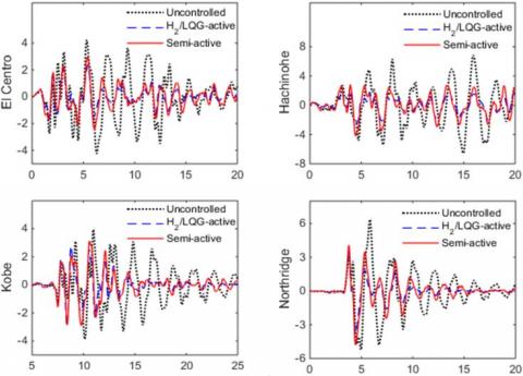
Table 2 provides the displacement responses and the VRRs of the target bridge under the four ground motions, considering hydrodynamic pressure. Figure 5 presents the time histories of pier-top displacement and bearing deformation under the four ground motions.
It can be seen that, considering the hydrodynamic pressure, the MR semi-active control reduced 21~40% of pier-top displacement and 50~69% of bearing deformation. The designed control force reduced the seismic responses to all four ground motions, showing a good control effect. Therefore, the MR semi-active control can effectively suppress the dynamic responses of the cross-sea bridge, enhancing the seismic safety of the bridge.
In addition, the time histories in Figure 5 show that the displacement responses of semi-active control and H2/LQG active control both declined significantly from the uncontrolled level, and the two control modes achieved very close results. This means the proposed MR semi-active control can track the optimal control force of the active control model in real time, an evidence of the effectiveness of the clipped-optimal algorithm. Hence, the MR damper provides a good alternative to the active control, if the latter is difficult to realize on bridge structures.
Table 2. Comparison of control effects considering hydrodynamic pressure
|
Maximum pier-top displacement / cm |
Maximum bearing deformation / cm |
|||||||||
|
Uncontrolled |
H2/LQG |
VRR (%) |
Semi-active |
VRR (%) |
Uncontrolled |
H2/LQG |
VRR (%) |
Semi-active |
VRR (%) |
|
|
El Centro |
4.25 |
2.38 |
44 |
2.97 |
30 |
7.92 |
3.41 |
57 |
3.41 |
57 |
|
Hachinohe |
6.85 |
3.32 |
52 |
4.11 |
40 |
11.26 |
6.95 |
38 |
3.46 |
69 |
|
JMA Kobe |
3.95 |
2.94 |
26 |
3.13 |
21 |
7.09 |
3.4 |
52 |
3.31 |
53 |
|
Northridge |
6.36 |
3.75 |
41 |
4.81 |
24 |
10.98 |
6.36 |
42 |
5.53 |
50 |
(a) Pier-top displacement (cm)
(b)Bearing deformation (cm)
Figure 5. The pier-top displacement and bearing deformation considering hydrodynamic pressure
(1) Considering the hydrodynamic pressure, it is learned that the presence of water changes the dynamic features of the structure, exerting a nonnegligible impact on the dynamic responses of the bridge structure.
(2) The presence of hydrodynamic pressure requires a higher semi-active control force. If hydrodynamic pressure is not considered in the control force design, the control force will be smaller than what is required, posing a security risk to the structure.
(3) The MR semi-active control can effectively suppress the dynamic responses of the cross-sea bridge, enhancing the seismic safety of the bridge.
(4) The semi-active controller, which is designed based on the clipped-optimal algorithm, achieved very close responses with the H2/LQG active control. This means the proposed semi-active controller can track the optimal control force of the active control model in real time, an evidence of the effectiveness of the clipped-optimal algorithm. Therefore, the MR damper provides a good alternative to the active control, if the latter is difficult to realize on bridge structures.
This work is supported by National Natural Science Foundation of China (Grant No.: 51678480).
[1] Li, Z.X., Wu, K., Shi, Y.D., Ning, L., Yang, D. (2019). Experimental study on the interaction between water and cylindrical structure under earthquake action. Ocean Engineering, 188: 106330. https://doi.org/10.1016/j.oceaneng.2019.106330
[2] Wang, Z.H., Gu, C.S., Chen, G.X. (2011). Seismic response of bridge pier in deep water considering close fluid-structure interaction effects. In Advanced Materials Research, 243: 1803-1810. https://doi.org/10.4028/www.scientific.net/AMR.243-249.1803
[3] Zhang, S., Tao, X., Liu, H. (2018). Seismic hydrodynamic pressure of bridge pier in deep water. In 2017 3rd International Forum on Energy, Environment Science and Materials (IFEESM 2017), pp. 1784-1787. https://doi.org/10.2991/ifeesm-17.2018.323
[4] Zhou, Y., Sun, L. (2018). Effects of high winds on a long-span sea-crossing bridge based on structural health monitoring. Journal of Wind Engineering and Industrial Aerodynamics, 174: 260-268. http://dx.doi.org/10.1016/j.jweia.2018.01.001
[5] Jiang, H., Wang, B., Bai, X., Zeng, C., Zhang, H. (2017). Simplified expression of hydrodynamic pressure on deepwater cylindrical bridge piers during earthquakes. Journal of Bridge Engineering, 22(6): 04017014. http://dx.doi.org/10.1061/(ASCE)BE.1943-5592.0001032
[6] Li, Y., Li, Z., Wu, Q. (2017). Experiment and calculation method of the dynamic response of deep water bridge in earthquake. Latin American Journal of Solids and Structures, 14(13): 2518-2533. http://dx.doi.org/10.1590/1679-78253872
[7] Nie, S., Ye, Z., Yong, W., Guo, K. (2018). Velocity & displacement-dependent damper: A novel passive shock absorber inspired by the semi-active control. Mechanical Systems and Signal Processing, 99: 730-746. https://doi.org/10.1016/j.ymssp.2017.07.008
[8] Liu, Y.F., Lin, T.K., Chang, K.C. (2018). Analytical and experimental studies on building mass damper system with semi-active control device. Structural Control and Health Monitoring, 25(6): e2154. https://doi.org/10.1002/stc.2154
[9] Saeid, P., Bahar, A., Solmaz, P. (2016). Semi-active control of vertical vibration of suspension bridges subjected to earthquake excitations using MR dampers and fuzzy logic. Sharif: Civil Enineering, 32(3): 43-54.
[10] Heo, G., Joonryong, J. (2014). Semi-active vibration control in cable-stayed bridges under the condition of random wind load. Smart Materials and Structures, 23(7): 075027. https://doi.org/10.1088/0964-1726/23/7/075027
[11] Li, Z.X., Yue, F.Q., Zhou, L. (2007). Semi-active control on seismic responses of vibration-insulated urban elevated bridges. China Civil Engineering Journal, (1): 42-48. https://doi.org/10.15951/j.tmgcxb.2007.01.008.
[12] Rojas, R.A., Carcaterra, A. (2018). An approach to optimal semi-active control of vibration energy harvesting based on MEMS. Mechanical Systems and Signal Processing, 107: 291-316. https://doi.org/10.1016/j.ymssp.2017.11.005
[13] Beji, S. (2019). Applications of Morison's equation to circular cylinders of varying cross-sections and truncated forms. Ocean Engineering, 187: 106156. https://doi.org/10.1016/j.oceaneng.2019.106156
[14] Yang, W., Li, Q. (2013). The expanded Morison equation considering inner and outer water hydrodynamic pressure of hollow piers. Ocean Engineering, 69: 79-87. https://doi.org/10.1016/j.oceaneng.2013.05.008
[15] Erkus, B., Abé, M., Fujino, Y. (2002). Investigation of semi-active control for seismic protection of elevated highway bridges. Engineering Structures, 24(3): 281-293. https://doi.org/10.1016/S0141-0296(01)00095-5
[16] Sun, J.Y., Yuan, Y.C., Li, K.P. (2011). Finite element program design of bridge structures with internal and external prestressing. In Advanced Materials Research, 250: 1493-1497. https://doi.org/10.4028/www.scientific.net/AMR.250-253.1493
[17] Dyke, S.J., Spencer Jr, B.F., Sain, M.K., Carlson, J.D. (1996). Modeling and control of magnetorheological dampers for seismic response reduction. Smart Materials and Structure, 5(5): 565-575. https://doi.org/10.1088/0964-1726/5/5/006
[18] Tan, P., Agrawal, A.K. (2009). Benchmark structural control problem for a seismically excited highway bridge - Part II: phase I sample control designs. Structural Control and Health Monitoring: The Official Journal of the International Association for Structural Control and Monitoring and of the European Association for the Control of Structures, 16(5): 530-548. https://doi.org/10.1002/stc.300
[19] Sodeyama, H., Sunakoda, K., Suzuki, K., Carlson, J.D., Spencer, B.F. (2001). Development of large capacity semi-active vibration control device using magneto-rheological fluid. American Society of Mechanical Engineers, Pressure Vessels and Piping Division (Publication) PVP, 428(2): 109-114.
[20] Yadi, S., Suhendro, B., Priyosulistyo, H., Aminullah, A. (2019). Dynamic response of long-span bridges subjected to nonuniform excitation: a state-of-the-art review. In MATEC Web of Conferences, 258: 05017. https://doi.org/10.1051/matecconf/201925805017
[21] Shi, L.L., Yao, S.C., Xuan, L.M., Dai, R. (2018). Experimental and numerical investigation of the wake structure and aerodynamic loss of trailing edge jet. Journal of Mechanical Science and Technology, 32(5): 2039-2046. https://doi.org/10.1007/s12206-018-0413-4