Mekonnen Shiferaw Ayano* | Olumuyiwa Otegbeye | Sicelo P. Goqo
© 2019 IIETA. This article is published by IIETA and is licensed under the CC BY 4.0 license (http://creativecommons.org/licenses/by/4.0/).
OPEN ACCESS
In this study, the problem of an electrically conducting and steady incompressible micropolar fluid with a natural convection boundary layer flow in a sphere in the presence of a strong magnetic field has been considered. This type of flow has many engineering applications, such as drying processes, electronic cooling, ceramic processing, heat exchanger devices and many more. The effect of radiation, chemical reaction, magnetic source; permeability and heat source/sink on the velocity, temperature and concentration profiles of the fluid flow in the medium are investigated. The governing equations describing the problem are transformed into non-dimensional partial differential equations. The equations are solved with the recently introduced multi-domain spectral quasilinearization method. The method involves the use of quasilinearization in linearizing nonlinear functions, a domain splitting approach to split the time interval into several sub-intervals and the Chebyshev spectral collocation method in solving the system. The results obtained suggest that the various parameters tested have a significant impact on various flow profiles. While the velocity and temperature of the fluid increases with an increase in the heat source parameter, the concentration of the fluid are observed to increase with an increase in the radiation and permeability parameters, respectively. Increase in the chemical reaction parameter leads to a decrease in the fluid velocity around the boundary layer. The analysis performed suggests that the multidomain spectral quasilinearization method is efficient in solving fluid flow problems of similar dynamics.
radiation effect, chemical reaction, magnetohydrodynamic, heat source and sink, quasilinearization
There has been widespread interest in the study of natural convection flow on a sphere. Heat exchanges by convection are important in some engineering applications such as food and polymer processing, turbomachinery, electrical devices, and thermal oil recovery. Flows of electrically conducting fluids in the presence of a magnetic field have received much attention by many researchers in recent years due to their importance from a technical point of view. The problems of free convection boundary layer flow over or on bodies of various shapes have been discussed by several researchers. Molla et al. [1] investigated the MHD natural convection flow on a sphere in the presence of heat generation and in this study they found that both the velocity and temperature profiles increased significantly when the heat generation parameter was increased. Hossain and Paul [2] examined the free convection from a vertical permeable cone with non-uniform surface temperature. Chen et al. [3] presented a numerical investigation for steady free convection inside a cavity filled with a porous medium. In this study, they presented isothermal and streamlines at different aspect ratios waviness, and Darcy-Rayleigh numbers. The influence of Hall current, ion slip and permeability on unsteady MHD Coutte-Poiseuille flow in a porous medium in the presence of moving transverse magnetic field was studied by Singh et al. [4]. They reported that in the case of pure fluid regime, suction tends to enhance fluid velocity in both the primary and secondary flow directions while injunction diminishes it.
Convective flow through porous medium plays an important role in diverse applications, such as in geothermal operations, petroleum industries, paper and textile coating, thermal insulation, cooling of modern electronic systems, design of solid-matrix heat exchangers, chemical catalytic reactors, and many others. Thorough discussions of these and other applications are available in the monographs by Ingham and Pop [5], Nield and Bejan [6] and others. Convective flows along different geometries have been considered by many previous authors due to their industrial applications, for example, the free convection from a heated sphere with a large Grashof number studied by Potter and Riley [7]. In this study, the boundary layer solution at the sphere surface was obtained numerically and they demonstrated how the solution fails as the upper stagnation point is approached, and the fluid erupts from the boundary layer to form the plume which develops over the sphere. Nagaraju et al. [8] studied the impact of mass transpiration on unsteady boundary layer flow of impulsive porous stretching. It was noted that the inverse Darcy number and suction/injection parameter significantly impacted on the velocity profile. MHD mixed bioconvection in a square porous cavity filled by gyrotactic microorganisms was examined by Mohamed et al. [9]. In this study, it was observed that natural convection increases and the transferred heat and mass-energy by convection equally increases. Hossain et al. [10] studied the conjugate effect of heat and mass transfer in natural convection flow from an isothermal sphere with chemical reaction. In this study, they analyzed the effects of the chemical reaction, buoyancy parameter, Schmidt and Prandtl number. Double-diffusion MHD free convective flow along a sphere in the presence of a homogeneous chemical reaction and Soret and Dufour effects were studied by Chamkha et al. [11]. The effect of thermal radiation, Soret and Dufour were reported in this study. Cattaneo-Christov heat flux model for chemically reacting radiative nanofluid flow over a cone or plate or wedge was studied by Chakravarthula et al. [12]. They observed that there were more reactions when studying heat and mass transport within a cone than between wedges and plates. Jasem [13] studied the conjugate free convective heat transfer behavior in an enclosure with two solid thick surfaces of walls in which the heat enters the enclosure from the bottom of the thick surface and leaves the enclosure from the top of another surface. In this study, it was reported that an increase in the Rayleigh number increased heat transfer.
Few works are available in the literature on the subject of free convection flow in porous media with MHD effects. In the various research reviewed and to the best of the authors knowledge, the combined effect of chemical reaction, thermal reaction heat sources/sink and permeability parameter on the motion of the fluid flow has not been studied. In the present paper, we study the simultaneous effect of the MHD free convection flow on a sphere through porous medium considering ohmic dissipation, chemical reaction, heat generation, and absorption. The non-dimensional equations are solved using the multidomain spectral quasilinearization method (MD-SQLM). The MD-SQLM, as introduced by Agbaje et al. [14] with the full description given by Goqo et al. [15], involves linearizing nonlinear functions using the quasilinearization method, introduced by Bellman and Kalaba [16]. The linearized system of equations is further split with respect to the domain of the tangential coordinate ξ into several sub-intervals by making use of non-overlapping grid-points. The ensuing system of linearized differential equations is solved using the Chebyshev spectral collocation method. Velocity, temperature and concentration distributions for the selected parameters studied.
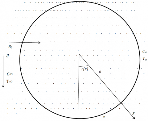
We consider the two-dimensional steady natural convection flow of an incompressible fluid flow over a sphere of radius a embedded in a porous medium. The surface is maintained at a uniform temperature Tw, which may either exceed the ambient temperature T∞ or may be less than T∞, Where the case Tw > T∞ is an upward flow along the surface due to free convection and Tw < T∞ is a downward flow. A sketch of the physical problem and the coordinate system are shown in Figure 1. Under the usual Boussinesq and boundary layer approximation, the basic equations are:
$\frac{\partial(r u)}{\partial x}+\frac{\partial(r v)}{\partial y}=0$ (1)
$\begin{aligned} \frac{1}{\epsilon^{2}}\left(u \frac{\partial u}{\partial x}+v \frac{\partial u}{\partial y}\right)=& v \frac{\partial^{2} u}{\partial y^{2}}-v \frac{u}{\kappa}-\frac{\sigma B_{0}^{2}}{\epsilon \rho} u+g^{*}\left[\beta_{T}\left(T-T_{\infty}\right)+\right.\\ &\left.\beta_{c}\left(C-C_{\infty}\right)\right] \sin \frac{x}{a} \end{aligned},$ (2)
$u \frac{\partial T}{\partial x}+v \frac{\partial T}{\partial y}=\alpha \frac{\partial^{2} T}{\partial y^{2}}+\frac{Q_{0}}{c_{p}}\left(T-T_{\infty}\right)-\frac{1}{\rho c_{p}} \frac{\partial q_{r}}{\partial y}+\frac{\sigma B_{0}^{2}}{\rho c_{p}} u^{2}$ (3)
$u \frac{\partial C}{\partial x}+v \frac{\partial C}{\partial y}=D_{m} \frac{\partial^{2} C}{\partial y^{2}}-K_{1}\left(C-C_{\infty}\right)$ (4)
where, u and v are velocity components in the x, y directions, ρ is the fluid density, T and C are temperature and concentrations, respectively, g∗ is the acceleration due to gravity, κ is the permeability of the porous medium, σ is electrical conductivity of the fluid, βT is the coefficient of thermal expansion, βc is the coefficient of solutal expansion, B0 magnetic field intensity, qr is radiative heat flux, α is the coefficient of thermal diffusivity, ν is kinematic viscosity of the fluid, Cp is the specific heat, Dm is the mass diffusivity, Q0 is heat generation (Q0 > 0) and or absorption (Q0 < 0) constant and K1 chemical reaction parameter.
Here, r=r(x)=a sin(x/a) is the radial distance from the symmetrical axis where a is the radius of the sphere. The boundary conditions are given by
u = 0, v = 0, T = Tw, C = Cw, on y = 0 (5a)
$u=0, T=T_{\infty,} \quad C=C_{\infty, \text { as }} \quad y \rightarrow \infty$ (5b)
Figure 1. Flow geometry
The radiative heat flux term is simplified by the Rosseland approximation as defined by Brewster [17]) as:
$q_{r}=-\frac{\sigma_{0}}{3 k^{*}} \frac{\partial \tau^{4}}{\partial y}$ (6)
where, σ0 is the Stephan-Boltzmann constant and k* is mean absorption coefficient. If the temperature differences within the flow are sufficiently small, T4 may be expanded by Taylor series. Hence, expanding T4 about T∞ and neglecting higher order terms we get
$T^{4} \cong T^{4} T_{\infty}^{4}+4\left(T-T_{\infty}\right) T_{\infty}^{3}=4 T_{\infty}^{3} T-3 T_{\infty}^{4}$ (7)
Using (7) Eq. (3) becomes
$u \frac{\partial T}{\partial x}+v \frac{\partial T}{\partial y}=\frac{k}{\rho c_{p}} \frac{\partial^{2} T}{\partial y^{2}}+\frac{Q_{0}}{c_{p}}\left(T-T_{\infty}\right)-\frac{16 \sigma^{*}}{3 k^{*} \rho C_{p}} \frac{\partial T}{\partial y}+\frac{\sigma B_{0}^{2}}{\rho c_{p}} u^{2}$ (8)
Introducing a stream function Ψ defined by $u=\frac{\partial \Psi}{\partial y}$ and $v=\frac{\partial \Psi}{\partial x}$ satisfying the mass conservation equation following the non-dimensional variables
$\begin{aligned} \xi &=\frac{\mathrm{x}^{1 / 2}}{\mathrm{L}^{1 / 2}}, \eta=\frac{\mathrm{yG}_{\mathrm{r}}^{1 / 4}}{\mathrm{a}}, \mathrm{U}=\mathrm{G}_{\mathrm{r}}^{-1 / 2} \mathrm{u}, \quad \mathrm{V}=\mathrm{G}_{\mathrm{r}}^{-1 / 4} \mathrm{v} \\ \theta &=\frac{T-T_{\infty}}{T_{w}-T_{\infty}}, \quad \phi(\xi, \eta)=\frac{c-c_{\infty}}{c_{w}-C_{\infty}}, \quad G_{r}=\frac{g^{*} \beta_{T}\left(T_{w}-T_{\infty}\right) a^{3}}{v^{2}} \end{aligned}$
$E_{c}=\frac{v^{2} G_{r}}{C_{p} a^{2}\left(T_{w}-T_{\infty}\right)}, \quad \operatorname{Pr}=\frac{\rho v C_{p}}{k}, \quad M=\frac{\sigma B_{0}^{2} a^{2}}{\rho v \mathbf{G}_{\mathbf{r}}^{1 / 2'}}$
$\delta=\frac{a^{2}}{\kappa \mathbf{G}_{\mathbf{r}}^{1 / 2}}, \quad \Delta=\frac{\beta_{c}\left(C_{w}-C_{\infty}\right)}{\beta_{T}\left(T_{w}-T_{\infty}\right)}, \quad \lambda=\frac{Q_{0} a^{2}}{\rho C_{p} v \mathbf{G}_{\mathbf{r}}^{1 / 2'}}$ (9)
$\mathrm{K}=\frac{k_{1} a^{2}}{v \mathbf{G}_{\mathrm{r}}^{1 / 2}}, \quad S c=\frac{v}{D_{m}}, \quad R d=\frac{k k^{*}}{3 \sigma_{0} T_{\infty}^{3}}$
where, M is the magnetic parameter, ξ is the dimensionless tangential coordinate, η is the dimensionless normal coordinate, Ec is the Eckert number, Rd is the radiation parameter, Gr is the local Grashof number, δ is the permeability parameter of the porous medium [18], λ is the heat source/sink parameter and K is the chemical reaction parameter.
Substituting Eq. (9) into Eqns. (1, 2, 8 and 4), the transformed equations are
$\frac{\partial(r U)}{\partial \xi}+\frac{\partial(r V)}{\partial \eta}=0$ (10)
$\frac{1}{\varepsilon^{2}}\left(U \frac{\partial U}{\partial \xi}+V \frac{\partial V}{\partial \eta}\right)=(\theta+\Delta \phi) \sin \xi+\frac{1}{\epsilon} \frac{\partial^{2} U}{\partial \eta^{2}}-\delta U-\frac{M}{\epsilon} U$ (11)
$U \frac{\partial \theta}{\partial \xi}+V \frac{\partial \theta}{\partial \eta}=\frac{1}{\operatorname{Pr}}\left(1+\frac{4}{3 R d}\right) \frac{\partial^{2} \theta}{\partial \eta^{2}}+\lambda \theta+M E c U^{2}$ (12)
$U \frac{\partial \phi}{\partial \xi}+V \frac{\partial \phi}{\partial \eta}=\frac{1}{S c} \frac{\partial^{2} \phi}{\partial \eta^{2}}-K \phi$ (13)
The corresponding transformed boundary conditions are
U = 0, V = 0, θ = 1, ϕ = 1 on η = 0 (14a)
U → 0, θ → 0, ϕ → 0 as η → ∞ (14b)
Introduce the non-dimensional stream function ψ = ξr(ξ)f(ξ,η) where U = $\frac{1}{r} \frac{\partial \psi}{\partial \eta}$ and V= $-\frac{1}{r} \frac{\partial \psi}{\partial \xi}$and inserting in (10-13), we obtain
$\begin{aligned} & \frac{1}{\epsilon^{2}} \frac{\partial^{3} f}{\partial \eta^{3}}+\frac{1}{\epsilon^{2}}\left(1+\frac{\xi \cos \xi}{\sin \xi}\right) f \frac{\partial^{2} f}{\partial \eta^{2}}-\frac{1}{\epsilon^{2}}\left(\frac{\partial f}{\partial \eta}\right)^{2} \\-\left(\delta-\frac{M}{\epsilon}\right) \frac{\partial f}{\partial \eta}+\frac{\sin \xi}{\xi}(\theta+\Delta \phi) &=\frac{\xi}{\varepsilon^{2}}\left(\frac{\partial f}{\partial \eta} \frac{\partial^{2} f}{\partial \eta \partial \xi}-\frac{\partial f}{\partial \xi} \frac{\partial^{2} f}{\partial \eta^{2}}\right) \end{aligned}$ (15)
$\begin{array}{c}{\frac{1}{P r}\left(1+\frac{4}{3 R d}\right) \frac{\partial^{2} \theta}{\partial \eta^{2}}+\left(1+\frac{\xi \cos \xi}{\sin \xi}\right) f \frac{\partial \theta}{\partial \eta}+\lambda \theta+} \\ {M E c \xi^{2}\left(\frac{\partial f}{\partial \eta}\right)^{2}=\left(\frac{\partial f}{\partial \eta} \frac{\partial \theta}{\partial \xi}-\frac{\partial f}{\partial \xi} \frac{\partial \theta}{\partial \eta}\right)}\end{array}$ (16)
$\frac{1}{s c} \frac{\partial^{2} \phi}{\partial \eta^{2}}+\left(1+\frac{\xi \cos \xi}{\sin \xi}\right) f \frac{\partial \phi}{\partial \eta}-K \phi=\left(\frac{\partial f}{\partial \eta} \frac{\partial \phi}{\partial \xi}-\frac{\partial f}{\partial \xi} \frac{\partial \phi}{\partial \eta}\right)$ (17)
The corresponding transformed boundary conditions are
f = f'= 0, θ= ϕ=1 when η =0 (18a)
f'→0, θ→0, ϕ→ 0 as η →∞ 0 (18b)
At the lower stagnation point (ξ = 0), the above equations reduced to the following ordinary differential equations.
$\frac{1}{\epsilon} f^{\prime \prime \prime}+\frac{2}{\epsilon^{2}} f f^{\prime \prime}-\frac{1}{\epsilon^{2}}\left(f^{\prime}\right)^{2}-\left(\delta+\frac{M}{\epsilon}\right) f^{\prime}+(\theta+\Delta \phi)=0$, (19)
$\frac{1}{\operatorname{Pr}}\left(1+\frac{4}{3 R d}\right) \theta^{\prime \prime}+2 f \theta^{\prime}+\lambda \theta+M E c\left(f^{\prime \prime}\right)^{2}=0$, (20)
$\frac{1}{s c} \phi^{\prime \prime}+2 f \phi^{\prime}-K \phi=0$, (21)
with the following boundary conditions to be solved
f=f'=0,θ=ϕ=1 when η = 0 (22a)
f'→0,θ→0,ϕ→0 as η → ∞ (22b)
In this section, we describe the application of the multi-domain spectral quasilinearization method (MD-SQLM) on the system of Eqns. (15)-(17). As previously described in Section 2, the MD-SQLM involves the application of quasilinearization on the nonlinear system and further solving the linearized system using Chebyshev spectral collocation method.
Linearizing the system of equations, we obtain
$\begin{aligned} \frac{1}{\epsilon} f_{r+1}^{\prime \prime \prime}+\left[a_{1}\right] f_{r+1}^{\prime \prime}+\left[a_{2}\right] f_{r+1}^{\prime}+\left[a_{3}\right] f_{r+1}+\left(\frac{\sin \xi}{\xi}\right) \theta_{r+1}+\\\left(\frac{\sin \xi}{\xi} \Delta\right) \phi_{r+1}=\left[a_{4}\right] \frac{\partial f_{r+1}^{\prime}}{\partial \xi}+\left[a_{5}\right] \frac{\partial f_{r+1}}{\partial \xi}+a_{6} \end{aligned},$ (23)
$\begin{aligned}\left[b_{1}\right] f_{r+1}^{\prime}+\left[b_{2}\right] f_{r+1}+\left[b_{3}\right] \theta_{r+1}^{\prime \prime}+\lambda \theta_{r+1} &=\left[b_{5}\right] \frac{\partial f_{r+1}}{\partial \xi} \\+\left[b_{6}\right] \frac{\partial \theta_{r+1}}{\partial \xi}+b_{7} \end{aligned},$ (24)
$\begin{aligned}\left[c_{1}\right] f_{r+1}^{\prime}+\left[c_{2}\right] f_{r+1}+\frac{1}{s c} \phi_{r+1}^{\prime \prime}+\left[c_{3}\right] \phi_{r+1}^{\prime}-K \phi_{r+1} &=\\\left[c_{4}\right] \frac{\partial f_{r+1}}{\partial \xi}+\left[c_{5}\right] \frac{\partial \phi_{r+1}}{\partial \xi} \end{aligned},$ (25)
where, the functions represented in closed brackets [...] represent vector functions and functions in open brackets (...) are scalar functions and
$a_{1}=\alpha_{1} f_{r}+\frac{\xi}{\epsilon^{2}} \frac{\partial f_{r}}{\partial \xi}, \quad a_{2}=-\frac{2}{\epsilon^{2}} f_{r+1}^{\prime}-\alpha_{3}-\frac{\xi}{\epsilon^{2}} \frac{\partial f_{r}^{\prime}}{\partial \xi}$,
$a_{3}=\alpha_{1} f_{r}^{\prime \prime}, \quad a_{4}=\frac{\xi}{\epsilon^{2}} f_{r}^{\prime}, \quad a_{5}=-\frac{\xi}{\epsilon^{2}} f_{r}^{\prime \prime}$,
$a_{6}=\alpha_{1} f_{r} f_{r}^{\prime \prime}-\frac{1}{\epsilon^{2}} f_{r}^{\prime 2}-\frac{\xi}{\epsilon^{2}} f_{r}^{\prime} \frac{\partial f_{r}^{\prime}}{\partial \xi}+\frac{\xi}{\epsilon^{2}} f_{r}^{\prime \prime} \frac{\partial f_{r}}{\partial \xi}$ ,
$b_{1}=2 M E c \xi^{2} f_{r}^{\prime}-\xi \frac{\partial \theta_{r}}{\partial \xi}, b_{2}=\alpha_{4} \theta_{r}^{\prime}$,
$\begin{aligned} b_{3}=\frac{1}{p r}\left(1+\frac{4}{3 R d}\right), b_{4}=& \alpha_{4} f_{r}+\xi \frac{\partial f_{r}}{\partial \xi}, b_{5}=-\xi \theta_{r}^{\prime}, b_{6}=\\ &-\xi f_{r}^{\prime} \\ b_{7}=\alpha_{4} f_{r} \theta_{r}^{\prime}+2 M E c \xi^{2} f_{r}^{\prime^{2}}-\xi f_{r}^{\prime} \frac{\partial \theta_{r}}{\partial \xi}+\xi \theta_{r}^{\prime} \frac{\partial f_{r}}{\partial \xi} \\ c_{1}=-\xi \frac{\partial \phi_{r}}{\partial \xi}, c_{2}=\alpha_{4} \phi_{r}^{\prime}, c_{3}=\alpha_{4} f_{r}+\xi \frac{\partial f_{r}}{\partial \xi} \\ c_{4}=-\xi \phi_{r}^{\prime}, c_{5}=-\xi f_{r}^{\prime}, c_{6}=\alpha_{4} f_{r} \phi_{r}^{\prime}-\xi f_{r}^{\prime} \frac{\partial \phi_{r}}{\partial \xi}+\xi \phi_{r}^{\prime} \frac{\partial f_{r}}{\partial \xi} \end{aligned}$,
where,
$\alpha_{1}=\frac{1}{\epsilon} \alpha_{4}=1+\frac{\xi \cos \xi}{\sin \xi}, \quad \alpha_{2}=\frac{1}{\epsilon^{2}}, \quad \alpha_{3}=\delta+\frac{M}{\epsilon}$
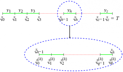
To solve the linearized system (24) which is defined in the tangential coordinate domain ξ ∈ [0, T], the interval is decomposed into z number of sub-intervals using the solutions from the previous interval in the next one. The figure below displays the decomposition process.
Figure 2. Non-overlapping multi-domain grid
The sub-intervals “y” of ξ, ξ = [0, T] given in Figure 2 are defined thus;
$y_{h}=\left(\xi_{h-1}, \xi_{h}\right), \quad h=1,2, \ldots, z, \text { where } 0=\xi_{0}, \xi_{1}, \ldots, \xi_{z}=T$. (26)
From the description given in (26), we obtain the system
$\begin{aligned} & \frac{1}{\epsilon} f_{r+1}^{\prime \prime \prime(h)}+\left[a_{1}^{(h)}\right] f_{r+1}^{\prime \prime(h)}+\left[a_{2}^{(h)}\right] f_{r+1}^{\prime}+\left[a_{3}^{(h)}\right] f_{r+1}^{(h)} \\+\left(\frac{\sin \xi}{\xi}\right) \phi_{r+1}^{(h)} &=\left[a_{4}^{(h)}\right] \frac{\partial f_{r}^{\prime(h)}}{\partial \xi}+\left[a_{5}^{(h)}\right] \frac{\partial f_{r}^{(h)}}{\partial \xi}+a_{6}^{(h)} \end{aligned}$, (27)
$\begin{aligned}\left[b_{1}^{(h)}\right] f_{r+1}^{\prime(h)}+\left[b_{2}\right] f_{r+1}^{(h)}+\left[b_{3}^{(h)}\right] \theta_{r+1}^{\prime \prime(h)}+\left[b_{4}^{(h)}\right] \theta_{r+1}^{\prime(h)}+\lambda \theta_{r+1}^{(h)} \\=\left[b_{5}^{(h)}\right] \frac{\partial f_{r+1}^{(h)}}{\partial \xi}+\left[b_{6}^{(h)}\right] \frac{\partial \theta_{r+1}^{(h)}}{\partial \xi}+b_{7}^{(h)} \end{aligned}$, (28)
$\begin{aligned}\left[c_{1}^{(h)}\right] f_{r+1}^{\prime(h)} &+\left[c_{2}\right] f_{r+1}^{(h)}+\frac{1}{S c} \phi_{r+1}^{\prime \prime(h)}+\left[c_{3}^{(h)}\right] \phi_{r+1}^{\prime(h)}-K \phi_{r+1}^{(h)} \\ &=\left[c_{4}^{(h)}\right] \frac{\partial f_{r+1}^{(h)}}{\partial \xi}+\left[c_{5}^{(h)}\right] \frac{\partial \phi_{r+1}^{(h)}}{\partial \xi} \end{aligned}$ (29)
It is important to note that the MD-SQLM requires initial solutions that satisfies the boundary conditions to solve the system (28). The process of continually using solutions from the previous sub-interval as initial solutions in the next sub-interval, referred to as a patching condition, is described by
$f^{(h)}\left(\eta, \xi_{h-1}\right)=f^{(h-1)}\left(\eta, \xi_{h-1}\right)$,
$\theta^{(h)}\left(\eta, \xi_{h-1}\right)=\theta^{(h-1)}\left(\eta, \xi_{h-1}\right)$,
$\phi^{(h)}\left(\eta, \xi_{h-1}\right)=\phi^{(h-1)}\left(\eta, \xi_{h-1}\right)$.
The linearized coupled system of Eqns. (27)-(29) is solved using the Chebyshev spectral collocation method. Detailed description about spectral methods can be obtained in Trefethen [19], Tang [20] and Canuto et al. [21]. Before solving the system, we use the physical transformations
$x=\frac{L_{x}}{2} \eta+\frac{L_{x}}{2} \& \quad y=\frac{L_{t}}{2} \xi+\frac{L_{t}}{2}$,
to transform the domains of η ∈[0,∞) and ξ ∈ [0,1] into x ∈ [−1,1] and y ∈ [−1,1], respectively. Lx and Ly are scaling parameters. Approximations of the solutions to f(x,t),θ(x,t) and ϕ(x,t) are expressed as Lagrange interpolating polynomials of the form
$f(x, t)=\sum_{i=0}^{M_{x}} \sum_{j=0}^{M_{y}} f\left(x_{i}, y_{j}\right) L_{i}(x) L_{j}(y),$
$\theta(x, t)=\sum_{i=0}^{M_{x}} \sum_{j=0}^{M_{y}} \theta\left(x_{i}, y_{j}\right) L_{i}(x) L_{j}(y),$ (30)
$\phi(x, t)==\sum_{i=0}^{M_{x}} \sum_{j=0}^{M_{y}} \phi\left(x_{i}, y_{j}\right) L_{i}(x) L_{j}(y)$, (31)
where, the Lagrange cardinal functions Li and Lj are defined as
$\begin{aligned} L_{i}^{(x)} &=\prod_{k=0}^{M_{x}} \frac{x-x_{k}}{x_{i}-x_{k}} \\ L_{j}^{(y)} &=\prod_{k=0}^{M} \prod_{k \neq j} \frac{y-y_{k}}{y_{j}-x_{k}} \end{aligned}$
and
$L_{i}\left(x_{k}\right)=\delta_{i k}=\left\{\begin{array}{l}{0 \text { if } i \neq k} \\ {1 \text { if } i=k'}\end{array}\right.$$L_{j}\left(y_{k}\right)=\delta_{j k}=\left\{\begin{array}{ll}{0} & {\text { if } j \neq k'} \\ {1} & {\text { if } j=k^{\prime}}\end{array}\right.$
where, the grid-points xi and yj are chosen to be Gauss-Chebyshev-Lobatto points obtained from
$\begin{aligned} x_{i} &=\cos \frac{\pi i}{M_{x}}, \quad \mathrm{i}=0,1, \ldots, M_{x} \\ y_{j} &=\cos \frac{\pi j}{M_{y}}, \quad \mathrm{i}=0,1, \ldots, M_{y} \end{aligned}$
To collocate the system (28), we use differentiation matrices (represented using D and d in x and y, respectively) defined as
$\left.\frac{\partial f^{(h)}}{\partial x^{(h)}}\right|_{x_{i}, y_{j}}=\boldsymbol{D}^{(h)} F_{i},\left.\quad \frac{\partial f}{\partial t}\right|_{x_{i}, y_{j}}=\sum_{j=0}^{M_{y}} d_{i j} F_{j},$
$\left.\frac{\partial \theta^{(h)}}{\partial x^{(h)}}\right|_{x_{i}, y_{j}}=D^{(h)} \theta_{i},\left.\quad \frac{\partial \theta}{\partial t}\right|_{x_{i}, y_{j}}=\Sigma_{j=0}^{M_{y}} d_{i j} \theta_{j}$,
$\left.\frac{\partial \phi^{(h)}}{\partial x^{(h)}}\right|_{x_{i}, y_{j}}=D^{(h)} \phi_{i},\left.\quad \frac{\partial f}{\partial t}\right|_{x_{i}, y_{j}}=\sum_{j=0}^{M_{y}} d_{i j} \Phi_{j},$ (32)
where, F, Θ and Φ are the vectors
$\boldsymbol{F}=\left[f\left(x_{0}, y_{j}\right), f\left(x_{1}, y_{j}\right), \ldots, f\left(x_{M_{x}}, y_{j}\right)\right]^{T}$,
$\boldsymbol{\theta}=\left[\theta\left(x_{0}, y_{j}\right), \theta\left(x_{1}, y_{j}\right), \ldots, \theta\left(x_{M_{x}}, y_{j}\right)\right]^{T}$,
$\boldsymbol{\phi}=\left[\phi\left(x_{0}, y_{j}\right), \phi\left(x_{1}, y_{j}\right), \ldots, \phi\left(x_{M_{x}}, y_{j}\right)\right]^{T}$,
where, T is the transpose. The representations given in (32) are applied in the coupled system (28) and we obtain the discretized system;
$\begin{array}{l}{\left[\frac{1}{\epsilon} \boldsymbol{D}^{3}+\left[a_{1, i}^{(h)}\right] \boldsymbol{D}^{2}+\left[a_{2, i}^{(h)}\right] \boldsymbol{D}+\left[a_{3, i}^{(h)}\right] \boldsymbol{F}_{r+1, i}^{(h)}-\right.} \\ {\left[\left(a_{4, i}^{(h)}\right] \sum_{j=0}^{M_{y}-1} \boldsymbol{d}_{i, j} \boldsymbol{D}+\left[a_{5, i}^{(h)}\right] \sum_{j=0}^{M_{y}-1} \boldsymbol{d}_{i, j}\right] \boldsymbol{F}_{r+1, j}^{(h)}+} \\ {\left[\left(\frac{\sin \xi}{\xi}\right) \boldsymbol{I}\right] \Theta_{r+1, i}^{(h)}+\left[\left(\frac{\sin \xi}{\xi} \Delta\right) \boldsymbol{I}\right] \Phi_{r+1, i}^{(h)}=R_{1, i}^{(h)}}\end{array}$ (33)
$\begin{aligned}\left[\left[b_{1, i}^{(h)}\right] \boldsymbol{D}+\left[b_{2, i}^{(h)}\right]\right] \boldsymbol{F}_{r+1, i}^{(h)}-\left[b_{5, i}^{(h)}\right] & \sum_{j=0}^{M_{y}-1} \boldsymbol{d}_{i, j} \boldsymbol{F}_{r+1, j}^{(h)} \\+&\left[\left[b_{3, i}^{(h)}\right] \boldsymbol{D}^{2}+\left[b_{4, i}^{(h)}\right] \boldsymbol{D}+\lambda \boldsymbol{I}\right] \Theta_{r+1, i}^{(h)}-\\\left[\boldsymbol{b}_{6, i}^{(h)}\right] \sum_{j=0}^{M_{y}-1} \boldsymbol{d}_{i j} \theta_{r+1, j}^{(h)} &=\boldsymbol{R}_{2, i}^{(h)} \end{aligned}$, (34)
$\begin{aligned}\left[\left[c_{1, i}^{(h)}\right] \boldsymbol{D}+\left[c_{2, i}^{(h)}\right]\right.& \boldsymbol{F}_{r+1, i}^{(h)}-\left[c_{4, i}^{(h)}\right] \sum_{j=0}^{M_{y}-1} \boldsymbol{d}_{i, j} \boldsymbol{F}_{r+1, j}^{(h)} \\ &+\left[\left(\frac{1}{S_{c}}\right) \boldsymbol{D}^{2}+\left[c_{3, i}^{(h)}\right] \boldsymbol{D}-K \boldsymbol{I}\right] \Phi_{r+1, i}^{(h)}-\\\left[\boldsymbol{c}_{5, i}^{(h)}\right] \sum_{j=0}^{M_{y}-1} \boldsymbol{d}_{i j} \Phi_{r+1, j}^{(h)} &=\boldsymbol{R}_{3, i}^{(h)} \end{aligned}$, (35)
where, I is an identity matrix of size (Mx + 1) × (Mx + 1) and
$\boldsymbol{R}_{1, i}^{(h)}=\boldsymbol{a}_{4, i}^{(h)} \boldsymbol{d}_{i, M_{y}}\left(D \boldsymbol{F}_{M_{y}}^{(h)}\right)+\boldsymbol{a}_{5, i}^{(h)} \boldsymbol{d}_{i, M_{y}} \boldsymbol{F}_{M_{y}}^{(h)}+\boldsymbol{a}_{6, i}^{(h)}$,
$\boldsymbol{R}_{2, i}^{(h)}=\boldsymbol{b}_{5, i}^{(h)} \boldsymbol{d}_{i, M_{y}} \boldsymbol{F}_{M_{y}}^{(h)}+\boldsymbol{b}_{6, i}^{(h)} \boldsymbol{d}_{i, M_{y}} \boldsymbol{\Theta}_{M_{y}}^{(h)}+\boldsymbol{b}_{7, i}^{(h)}$,
$\boldsymbol{R}_{3, i}^{(h)}=\boldsymbol{c}_{4, i}^{(h)} \boldsymbol{d}_{i, M_{y}} \boldsymbol{F}_{M_{y}}^{(h)}+\boldsymbol{c}_{5, i}^{(h)} \boldsymbol{d}_{i, M_{y}} \mathbf{\Phi}_{M_{y}}^{(h)}+\boldsymbol{c}_{6, i}^{(h)}$.
In this section, we present the numerical solutions to the system of Eqns. (33)-(35). The effect of increasing the dimensionless tangential coordinate ξ, radiation parameter Rd, chemical reaction parameter K and the heat source\sink parameter λ on the velocity, temperature and concentration flow profiles of the micropolar fluid in the porous medium. The MD-SQLM is tested to verify that the solutions obtained to the problem defined by (33)-(35) are convergent given a certain tolerance level and the solutions display a high level of accuracy. To carry out this study, we used 50 grid points in η, 10 grid points in ξ and the domain of the tangential coordinate was split into 9 sub-intervals. These points were observed to produce accurate solutions and increase of the grid points did not improve the speed of convergence or accuracy of the solutions obtained.
To investigate the speed of convergence of solutions obtained using the MD-SQLM to some certain tolerance level, the solution error is calculated using the difference between solutions after successive iterations. At the point where a further increase in iterations does not change the error significantly, we conclude convergence of the method. The solution error norms are obtained using
$\|\boldsymbol{F}\|_{\infty}=\max _{0 \leq i \leq M_{t}}\left\|\boldsymbol{F}_{r+1, i}-\boldsymbol{F}_{r, i}\right\|_{\infty}$,
$\|\mathbf{\Theta}\|_{\infty}=\max _{0 \leq i \leq M_{t}}\left\|\Theta_{r+1, i}-\Theta_{r, i}\right\|_{\infty}$,
$\|\Phi\|_{\infty}=\max _{0 \leq i \leq M_{t}}\left\|\Phi_{r+1, i}-\Phi_{r, i}\right\|_{\infty}$. (36)
Figures 3a to 3c display the speed of convergence of solutions using the MD-SQLM. The Figures are obtained when $\delta=10 e 4, \epsilon=1, P r=0.72, M=2, R d=2, \lambda=$$0.5, E c=0.01, \Delta=2, K=2 \text { and } S c=0.22$.
From Figures 3a to 3c, it is observed that as the number of iterations increase, the solution errors reduce until after the fifth iteration where they seem to reach a plateau. This indicates that the MD-SQLM is convergent from problems of this nature. From the slope of the curves in the Figures, we observe that the solutions converge quadratically. This is as a
result of the method having similar characteristics to the well known Newton-Rhapson method.
Figure 3. Effect of iterations on the error norms when ξ = 1.5
The quadratic convergence implies that that MD-SQLM, whenever it gives convergent solutions, will always converge rapidly after few iterations. Exception will occur when emphasis is placed on digit precision of the method and set to be very high. This will result in increasing the number of iterations before convergence but on the positive note, exponentially reduce the solution error obtained. We note that the digit precision used for this study was set as 30 and the software used was Mathematica. To study the accuracy of solutions obtained using the MD-SQLM, the residual error norm is obtained by representing the system of Eqns. (33)-(35) with the approximated solutions obtained. The size of the error obtained gives an indication as to how accurate the MD-SQLM is when solving similar problems. The residual error norms are calculated thus;
$\begin{aligned} \operatorname{Res}(\boldsymbol{F})=& \max _{0 \leq i \leq M_{y}} \| \frac{1}{\epsilon} \boldsymbol{f}_{i}^{\prime \prime \prime}+\frac{1}{\epsilon^{2}}\left(1+\frac{\xi \cos \xi}{\sin \xi}\right) \boldsymbol{f}_{i} \boldsymbol{f}_{i}^{\prime \prime}-(\delta+\\\left.\frac{M}{\epsilon}\right) \boldsymbol{f}_{i}^{\prime}+\frac{\sin \xi}{\xi}\left(\boldsymbol{\theta}_{i}+\Delta \boldsymbol{\phi}_{i}\right)-\frac{\xi}{\epsilon^{2}}\left(\boldsymbol{f}_{i}^{\prime} \frac{\partial \boldsymbol{f}_{i}^{\prime}}{\partial \xi}-\boldsymbol{f}_{i}^{\prime \prime} \frac{\partial f_{i}}{\partial \xi}\right) \|_{\infty} \end{aligned}$, (37)
$\begin{aligned} \operatorname{Res}(\mathbf{\Theta}) &=\max _{0 \leq i \leq M_{y}} \| \frac{1}{\operatorname{Pr}}\left(1+\frac{4}{3 R_{d}}\right) \boldsymbol{\theta}_{i}^{\prime \prime}+\left(1+\frac{\xi \cos \xi}{\sin \xi}\right) \boldsymbol{f}_{i} \boldsymbol{\theta}_{i}^{\prime}+\\ \lambda \boldsymbol{\theta}_{i}+M \operatorname{Ec} \xi^{2} \boldsymbol{f}_{i}^{\prime 2}-& \xi\left(\boldsymbol{f}_{i}^{\prime} \frac{\partial \boldsymbol{\theta}_{i}}{\partial \xi}-\boldsymbol{\theta}_{i}^{\prime} \frac{\partial f_{i}}{\partial \xi}\right) \|_{\infty} \end{aligned}$ (38)
$\begin{aligned} \operatorname{Res}(\mathbf{\Phi})=& \max _{0 \leq i \leq M_{y}} \| \frac{1}{S c} \boldsymbol{\phi}_{i}^{\prime \prime}+\left(1+\frac{\xi \cos \xi}{\sin \xi}\right) \boldsymbol{f}_{i} \boldsymbol{\phi}_{i}^{\prime}-K \boldsymbol{\phi}_{i} \\ &-\xi\left(\boldsymbol{f}_{i}^{\prime} \frac{\partial \boldsymbol{\phi}_{i}}{\partial \xi}-\boldsymbol{\phi}_{i}^{\prime} \frac{\partial \boldsymbol{f}_{i}}{\partial \xi}\right) \|_{\infty} \end{aligned}$.
Figures 4a to 4c display the residual error norms of the approximate solutions obtained using the MD-SQLM to the Eqns. (33)-(35).
Figure 4. Effect of iterations on the residual error norms when ξ = 1.5
Figures 4a to 4c show that the approximate solutions obtained using the MD-SQLM leave small errors. As displayed in Figure 4a, the residual error norm is consistent at 10−12. This is because equation (33) is nonlinear in f and its derivatives only and hence, the solutions for θ and φ are always known when that equation is being solved. It is also observed from Figures 4b and 4c that as the number of iterations increase, the residual error norms decrease and plateau out after the 3rd iteration to an error of 10−34. We see from these figures that the MD-SQLM is highly accurate when solving problems of similar nomenclature to the one under investigation in this study.
We proceed to study the effect of certain parameters on the flow profiles. Unless where varied, the study is conducted at the fixed values $\delta=1, \epsilon=1, \operatorname{Pr}=0.72, M=1, R_{d}=1.5, \lambda=0.1, E c=1, \Delta=2, K=1, \text { and } S c=0.22$.
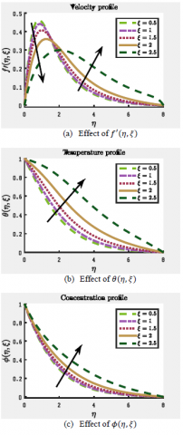
Figures 5a to 5c display the effect of the dimensionless tangential coordinate ξ on the velocity, temperature and concentration profiles.
Figure 5. Effect of tangential coordinate ξ
It is observed in Figure 5a that as the normal coordinate η increases from 0 to 2, an increase in the tangential coordinate ξ decreases the velocity profile but increases the profile for 2 < η ≤ 8. In Figures 5b and 5c, it is seen that an increase in ξ increases both the temperature and concentration profile.
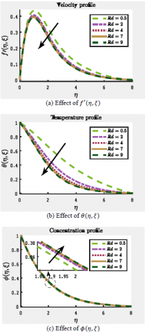
Figures 6a to 6c display the effect of increasing radiation on the flow profiles.
Figure 6. Effect of radiation Rd
As shown in Figures 6a and 6b, an increase in radiation decreases the velocity and the temperature profiles, however, Figure 6c shows an increase in concentration when Rd is increased. When radiation is present, the thermal boundary layer was always found to thicken, which may be explained by the fact that radiation provides an additional means to diffuse energy.
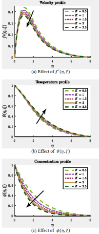
In Figures 7a to 7c, the effect of increasing chemical reaction on the flow profiles are displayed.
Figure 7: Effect of chemical reaction K From Figures 7a and 7c, it is observed that as chemical reaction increases, velocity and concentration decreases while temperature increases as displayed in Figure 7b.
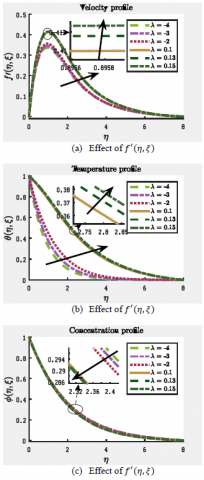
Figures 8a to 8c display the effect of heat source on the profiles.
Figure 7. Effect of chemical reaction K
From Figures 8a and 8b, it is observed that as the amount of heat let into the medium increases, the fluid heats up thereby increasing the temperature of the medium and increasing the movement of the fluid. Expectedly, this reaction causes some of the fluid to vaporize thereby decreasing the concentration of the fluid in the medium as shown in Figure 8c. Physically, the higher values of ν in the equations $G r=\frac{g^{*} \beta_{T}\left(T_{w}-T_{\infty}\right) a^{3}}{v^{2}}$ , and $\mathrm{K}=\frac{k_{1} a^{2}}{v \mathrm{c}_{\mathrm{r}}^{1 / 2}}$ make fall in the chemical molecular diffusivity. An increase in the chemical reaction parameter will suppress species concentration. On the other hand, the energy is absorbed by decreasing the values of heat sink parameter resulting in the temperature to drop near the boundary layer.
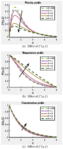
Figures 9a to 9c display the effect of the permeability parameter δ on the various fluid flow profiles.
Figure 8. Effect of heat source λ
Figure 9. Effect of permeability δ
As shown in Figure 9a, an increase in the permeability of the wall of the porous medium significantly decreases the velocity of the fluid. However, as displayed in Figures 9b and 9c, an increase in δ increases the temperature and concentration of the fluid in the porous medium.
This paper presents the simultaneous effect of the MHD free convection flow on a sphere through porous medium considering ohmic dissipation, chemical reaction, heat generation, and absorption. The effect of tangential coordinate, radiation, chemical reaction, heat source/sink and permeability on the velocity, temperature and concentration flow profiles have been investigated. The results were obtained using the multi-domain spectral quasilinearization method. The key findings of the study include;
Contribution of chemical reaction, thermal reaction heat sources/sink and permeability parameter on the motion of the fluid flow are significant and they cannot be ignored.
In this study, we assumed the magnetic field strength to be low so that the Hall and ion-slip effects are neglected. The relationship between the fluxes and the driving potentials are also not considered. The future work will include these and other similar parameter influence on the flow.
|
u, v T C |
Velocity components Temerature Concentration |
|
CP |
specific heat, J. kg-1. K-1 |
|
g* |
gravitational acceleration, m.s-2 |
|
A x, y r U,V Pr M |
Radius of a sphere coorinates axes radial distance diamensionless coordinates Prandtl number Magnatic parameter |
|
Greek symbols
|
|
|
a |
thermal diffusivity, m2. s-1 |
|
bT |
thermal expansion coefficient, K-1 |
|
β |
Casson parameter |
|
f |
solid volume fraction |
|
Ɵ |
dimensionless temperature |
|
µ |
dynamic viscosity, kg. m-1.s-1 |
|
ρ $β_C$ |
fluid density coefficient of expansion with concentration |
|
$σ_0$ |
Stephan-Boltzmann constant |
|
Subscripts |
|
|
K* |
mean absorption parameter |
|
Grx |
local Grashof number |
|
$T_∞$ |
Ambient temperature |
|
Q0 |
Heat generation/absorption parameter |
|
B0 |
strength of the magnetic field |
|
Tw |
surface temperature |
[1] Molla, M.M., Taher, M.A., Chowdhury, M.M.K., Hossain, M.A. (2005). Magnetohydrodynamic natural convection flow on a sphere in presence of heat generation. Nonlinear Analysis: Modelling and Control, 10(4): 349-363. https://doi.org/10.1007/s00707-006-0373-0
[2] Hossain, M.A., Paul, S.C. (2001). Free convection from a vertical permeable cone with nonuniform surface temperature. Acta Mechanica, 151: 103-114. https://doi.org/10.1007/BF01272528
[3] Chen, X.B., Yu, P., Winoto, S.H., Low, H.T. (2007). Free convection in a porous wavy cavity based on the Darcy– Brinkman–Forchheimer extended model. Numer. Heat Transf., Part A: Applications, 52: 377-397. https://doi.org/10.1080/10407780701301595
[4] Singh, J.K., Naveeen, J., Ghousia, B. (2016). Unsteady magnetohydrodynamic Couette-Poiseuille flow within porous plate filled with porous medium in the presence of a moving magnetic field with Hall and ion-slip effects. Int. J. of Heat and Technology, 34(1): 89-97. https://doi.org/10.18280/ijht.340113
[5] Ingham, D.B., Pop, I. (2002). Transport phenomena in porous media II pergamon, Oxford (2002).
[6] Nield, D.A., Bejan, A. (2006). Convection in Porous Media. 3rd edition, Springer, New York.
[7] Potter, J.M., Riley, N. (1980). Free convection from a heated sphere at large Grashof number. J. of Fluid Mech., 100(4): 769-783. https://doi.org/10.1017/S0022112080001395
[8] Nagaraju, K.R., Mahabaleshwar, U.S., Krimpeni, A.A., Ioannis, E., Lorenzini, G. (2019). The impact of mass transpiration on unsteady boundary layer flow of impulsive porous stretching. Mathematical Modelling of Engineering Problems, 6(3): 349-354. https://doi.org/10.18280/mmep.060305
[9] Mohamed, A.M., Ahmed, M.R., Bandaru, M., Ahmed, K.H., Mohamed, A., Lioua, K. (2019). MHD Mixed bioconvection in a square porous cavity filled by gyrotactic microoorganisms. Int. J. of Heat and Technology, 37(2): 433-445. https://doi.org/10.18280/ijht.370209
[10] Hossain, M.A., Molla, M.M., Gorla, R.S.R. (2004). Conjugate effect of heat and mass transfer in natural convection flow from an isothermal sphere with chemical reaction. Int. J. Fluid Mech. Research, 31(4): 104-117. https://doi.org/10.1615/InterJFluidMechRes.v31.i4.20
[11] Chamkha, A.J., Aly, A.M., Raizah, Z.A.S. (2017). Double Diffusion MHD free convective flow along a sphere in the presence of a homogeneous chemical reaction and Soret and Dufour effects. Applied and Computational Math, 6(1): 34-44. http://doi:10.11648/j.acm.20170601.12
[12] Chakravarthula, S.K., Naramgari, S., Lorenzini, G., Mohammad, H.A. (2018). Chemically reacting Carreau fluid in a suspension of convictive conditions over three geometries with Cattaneo-Chritov heat flux model. Mathematical Mod. of Eng. Problems, 5(4): 292-302. http://doi.org/10.18280/mmep.050404
[13] Jasem, M.A. (2019). Non-equilibrium natural convection flow through a porous medium. Mathematical Mod. of Eng Problems, 6(2): 163-169. http://doi/10.18280/mmep.060202
[14] Agbaje, T.M., Mondal, S., Motsa, S.S., Sibanda, P. (2017). A numerical study of unsteady non-Newtonian Powell-Eyring nanofluid over a shrinking sheet with heat generation and thermal radiation. Alexandria Engineering Journal, 56(1): 81-91. http://dx.doi.org/10.1016/j.aej.2016.09.006
[15] Goqo, S.P., Mondal, S., Sibanda, P., Motsa, S.S. (2019). Efficient multidomain spectral collocation solution for MHD laminar natural convection flow from a vertical permeable flat plate with uniform surface temperature and thermal radiation. International Journal of Computational Methods, 16(6): 1840029-46. https://doi.org/10.1142/S0219876218400297
[16] Bellman, R.E., Kalaba, R.E. (1965). Quasilinearization and nonlinear boundaryvalue problems. RAND Corporation, Santa Monica.
[17] Brewster, M.Q. (1992). Thermal Radiative Transfer Properties. John Wiley and Sons, Canada.
[18] Cortell, R. (2005). Flow and heat transfer of a fluid through a porous medium over a stretching surface with internal heat generation/absorption and suction/blowing. Fluid Dynamics Research, 37: 231-245. https://doi.org/10.1016/j.fluiddyn.2005.05.001
[19] Trefethen, L.N. (2000). Spectral Methods in MATLAB. Society for Industrial and Applied Mathematics, Philadelphia.
[20] Tang, T. (2006). Spectral and High-Order Methods with Applications. Science Press, Beijing.
[21] Canuto, C., Husseini, M.Y., Quarteroni, A., Zang, T.A. (1988). Spectral Methods in Fluid Dynamics. Springer-Verlag, Berlin, 1988.