OPEN ACCESS
In this article, the laminar mixed convective flow of an incompressible chemically reacting nanofluid in an annulus between two concentric cylinders is investigated by considering the Joule heating effect. The nonlinear governing equations are non-dimensionalized and then solved by using homotopy analysis method. The rate of entropy generation and Bejan number are calculated numerically. The effect of magnetic, Joule heating, Brinkman number and chemical reaction parameters on the velocity, temperature and nanoparticle concentration are investigated, and presented graphically. The maximum values of Bejan number Be are observed at the center of the annulus due to more contribution of heat transfer irreversibility on entropy generation and minimum value is near the cylinders, due to more contribution of fluid friction irreversibility on entropy generation with an increase in K, M, Br, J and Nt.
entropy generation, chemical reaction, HMD, nanofluid, concentric cylinders, joule heating effect, HAM
The study of a nanofluid flow has been attracted by the several researchers over the past decade. Nanofluids are convective heat transfer fluids containing suspensions of nanometer sized particles [1]. It is reported experimentally that these fluids possess substantially higher thermal conductivity proportionate to the base fluids [1]. Nanofluids have several applications in engineering, microfluidics, microelectronics, biomedical, manufacturing, solid-state lighting, transportation, scientific measurement, material synthesis, high-power X-rays, material processing and medicine. Further, the study of mixed convective heat transfer and nanofluid flow between concentric cylinders has acquired considerable attention due to its diverse application in the designs of cooling devices for electronica and microelectronic equipment, solar energy collection, etc. Several studies were conducted on the convective heat transfer and nanofluid flow through concentric cylinders by considering distinct types of conventional base fluids with particular nanoparticles. Sheikhzadeh et al [2] analyzed the mixed convective nanofluid in an annulus between concentric cylinders. Togun et al [3] presented a detailed review on heat transfer of mixed, forced and natural and convective nanofluid flow through various annular passage configurations. On the other hand, numerous researches have been carried out to study the influence of Joule heating on heat transfer and fluid flow under various conditions and found that it plays a notable effect on magnetohydrodynamics (MHD) flow and heat transfer. Nandkeolyar et al [4] focused on the effects of viscous dissipation and Joule heating on nanofluid flow through a shrinking/stretching sheet considering homogeneous and heterogeneous reactions. Zhang et al [5] conducted a numerical study on MHD fluid flow and heat transfer in a cavity under influence of Joule heating. Hayat et al [6] studied the mixed convective Jeffrey nanofluid flow in a compliant wall channel by taking Joule heating along with viscous.
The impact of chemical reaction on heat and mass transfer is of great influence in chemical technology and industries of hydrometallurgy. Chemically reacting nanofluid may play a significant role in many processing systems and materials. A number of researchers have focused on the chemical reaction effect on the heat and mass transfer flow passing through the annular region between concentric cylinders. Babulal and Dulal Pal [7] studied the combination of Joule heating and chemical reaction effects on the MHD mixed convective flow of a viscous fluid between vertical parallel plates. Mridul Kumar et al [8] analyzed the effect chemical reaction on MHD boundary layer flow over the stretching sheet with Joule heating effect. Poulomi et al [9] examined the significance of mixed convective chemically reacting nanofluid flow with internal heat generation and thermal radiation.
The irreversibility associated with the real processes is measured by entropy generation. When entropy generation takes place the quality of energy decreases i.e. the entropy generation destroys the system energy. Hence, the performance of the system can be improved by decreasing the entropy generation. Therefore, a powerful and useful optimization tool for a high range of thermal applications is minimization of entropy generation. Bejan [10, 11] developed the entropy generation optimization method and introduced its applications in science and engineering field. Since then several researchers have studied the entropy generation analysis for different types of geometries with diverse fluids. Gyftopoulos and Beretta [12] studied the entropy generation due to chemically reacting system. Miranda [13] analyzed entropy generation due to chemically reacting fluid flow. Imen et al [14] analyzed the entropy generation analysis of a chemical reaction process. Govindaraju et al [15] investigated the entropy generation analysis of magnetohydrodynamic flow of a nanofluid. Rashidi et al [16] presented the entropy generation on the MHD blood flow of a nanofluid influenced by the thermal radiation. Fersadou et al [17] analyzed numerically the entropy generation and MHD mixed convective nanofluid flow in a vertical channel. Omid et al [18, 19] analyzed the significance of radiation effect on entropy generation between two rotating cylinders using nanofluid. Dehsara et al [20] analyzed numerically the entropy generation in a nanofluid flow considering viscous dissipation and variable magnetic field. Srinivasacharya and Hima Bindu [21] studied the entropy generation in a micropolar fluid flow between concentric cylinders. Bouchoucha and Rachid [22] investigated the natural convection and entropy generation of nanofluid in a square cavity. Pooja et al [23] analyzed the entropy generation on forced convective flow of viscous fluid flow through a circular channel filled with a hyper porous medium saturated with a rarefied gas in the presence of transverse magnetic field, thermal radiation and uniform heat flux at the walls of the channel.
In most of the studies, reported in the literature, on mixed convective flow and heat transfer between concentric cylinders, the interactions of chemical reaction and Joule heating with nanoparticles and entropy generation have not been considered. The main aim of this study is to examine the combined effect of Joule heating and chemical reaction on MHD mixed convection flow and entropy generation due to nanofluid between concentric cylinders. The homotopy analysis method (HAM) is used to solve the nonlinear differential equations. HAM [22] was first introduced by Liao, which is one of the most powerful technique to find the solution of strongly nonlinear equations. The effect of Joule heating and chemical reaction on the temperature, velocity, nanoparticle concentration, Bejan number and entropy generation are investigated.
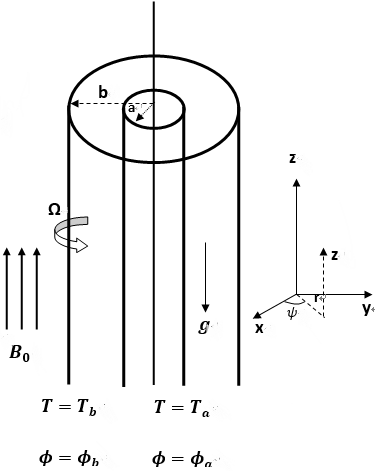
Consider steady, laminar and incompressible nanofluid flow in an annular space between two infinitely long concentric cylinders of radius ‘a’ and ‘b’ (a < b) and kept at temperatures Ta and Tb respectively. Choose cylindrical polar coordinates system $(r, \psi, z)$ with z-axis along the common axis of cylinders (as shown in Figure 1) and ‘r’ normal to the z-axis. Assume that the outer cylinder is rotating with a constant angular velocity Ω whereas the inner cylinder is at rest. The flow is induced due to the rotation of the exterior cylinder. A strong magnetic field B0 is taken in an axial direction. The conductivity of fluid is chosen to be small so that the magnetic Reynolds number is very smaller than one unit and hence the induced magnetic field is removable compared to the applied radial field. Thermophysical characteristics of the nanofluid are taken as constant except density in the buoyancy term of the balance of momentum equation. In addition, the thermophoresis and Brownian motion effects are incorporated [23]. The velocity component along $\Psi$ direction, temperature and nanoparticle concentration are denoted by u, T and f, respectively. The equations which govern the present flow [23] with Boussinesq approximation are
$\frac{\partial u}{\partial \psi}=0$ (1)
$\frac{\partial p^{*}}{\partial r}=\frac{u^{2}}{r}$ (2)
$\mu \nabla_{1}^{2} u+(1-\phi) \rho_{f} g \beta_{T}\left(T-T_{a}\right)$ $-\left(\rho_{p}-\rho_{f}\right) g\left(\phi-\phi_{a}\right)-\sigma B_{0}^{2} u-\frac{1}{r} \frac{\partial p^{*}}{\partial \psi}=0$ (3)
Figure 1. Geometry of the problem
$\alpha\left[\frac{\partial^{2} T}{\partial r^{2}}+\frac{1}{r} \frac{\partial T}{\partial r}\right]+\frac{\mu}{\rho c_{p}}\left[\left(\frac{\partial u}{\partial r}\right)^{2}-2 \frac{u}{r} \frac{\partial u}{\partial r}+\left(\frac{u}{r}\right)^{2}\right]+\frac{1}{\rho c_{p}} \sigma B_{0}^{2} u^{2}$ $+\tau\left[D_{B} \frac{\partial T}{\partial r} \frac{\partial \phi}{\partial r}+\frac{D_{T}}{T_{m}}\left(\frac{\partial T}{\partial r}\right)^{2}\right]=0$ (4)
$D_{B}\left[\frac{\partial^{2} \phi}{\partial r^{2}}+\frac{1}{r} \frac{\partial \phi}{\partial r}\right]+\frac{D_{T}}{T_{m}}\left[\frac{\partial^{2} T}{\partial r^{2}}+\frac{1}{r} \frac{\partial T}{\partial r}\right]$ $-k_{1}\left(\phi-\phi_{a}\right)=0$ (5)
where σ is the electrical conductivity, $\rho$ is the density, p* is the pressure, μ is the viscosity coefficient, DB is Brownian diffusion coefficient, D is the mass diffusivity, Tm is the mean fluid temperature, α is the effective thermal diffusivity, Cp is the specific heat capacity, βT is the coefficients of thermal expansion, DT is the thermophoresis diffusion coefficient, g is the acceleration due to gravity, $K_{f}=\alpha\left(\rho C_{p}\right)$ is the coefficient of thermal conductivity, k1 is the rate of chemical reaction, τ is the fraction of heat capacity of the fluid and effective heat capacity of the nanoparticle material and $\nabla_{1}^{2} u=\frac{\partial}{\partial r}\left[\frac{1}{r} \frac{\partial}{\partial r}(r u)\right]$ .
The conditions on the boundary are:
$u=0, T=T_{a}, \phi=\phi_{a}$ at $r=a$
$u=b \Omega, T=T_{b}, \phi=\phi_{b}$ at $r=b$ (6)
Introducing the following non-dimensional variables
$\lambda=\frac{r^{2}}{b^{2}}, f(\lambda)=\frac{u \sqrt{\lambda}}{b \Omega}, \theta=\frac{T-T_{a}}{T_{b}-T_{a}}$
$S=\frac{\phi-\phi_{a}}{\phi_{b}-\phi_{a}}, P=\frac{p^{*}}{\mu \Omega}$ (7)
in equations (1)-(5), we get the nonlinear differential equations as
$4 f^{\prime \prime} \lambda+\sqrt{\lambda} \frac{G r}{R e}(\theta-N r S)-M^{2} f-A=0$ (8)
$\left(\lambda^{3} \theta^{\prime \prime}+\lambda^{2} \theta^{\prime}\right)+B r\left[\lambda^{2}\left(f^{\prime}\right)^{2}-2 \lambda f f^{\prime}+(f)^{2}\right]$ $+\frac{1}{4} J \lambda^{2} f^{2}+\operatorname{Pr} N b \lambda^{3} \theta^{\prime} S^{\prime}+\operatorname{Pr} N t \lambda^{3}\left(\theta^{\prime}\right)^{2}=0$ (9)
$\lambda S^{\prime \prime}+S^{\prime}+\frac{N t}{N b}\left(\lambda \theta^{\prime \prime}+\theta^{\prime}\right)-\frac{K}{4} L e S=0$ (10)
where prime indicate the derivative corresponding to λ, the Prandtl number is $P r=\frac{\mu C_{p}}{k_{f}}$ , Grashof number is $G r=\frac{(1-\emptyset) g \beta_{T}\left(T_{b}-T_{a}\right) b^{3}}{v^{2}}$ , Reynold's number is $R e=\frac{\rho \Omega b^{2}}{\mu}$ ,constant pressure gradient is $A=\frac{\partial P}{\partial \varphi}$ , magnetic parameter is $M^{2}=\frac{\sigma B_{o}^{2} b^{2}}{\mu}$ , Brinkman number is $B r=\frac{\mu \Omega^{2}}{k_{f}\left(T_{b}-T_{a}\right) b^{2}}$, Brownian motion parameter is $N b=\frac{\tau D_{B}\left(\phi_{b}-\phi_{a}\right)}{v}$ , thermoporesis parameter is $N t=\frac{\tau D_{T}\left(T_{b}-T_{a}\right)}{T_{m} v}$ , buoyancy ratio is $N r=\frac{\left(\rho_{p}-\rho_{f}\right)\left(\phi_{b}-\phi_{a}\right)}{\rho_{f} \beta_{T}\left(T_{b}-T_{a}\right)(1-\phi)}$ , the chemically reacting parameter is $K=\frac{k_{1} b^{2}}{v}$ , Lewis number is $L e=\frac{v}{D_{B}}$ and Joule heating parameter is $J=\frac{\sigma B_{o}^{2} b^{2} \Omega^{2}}{\left(T_{b}-T_{a}\right) k_{f}}$ .
The corresponding conditions (7) on boundary are
$S=0, \theta=0, f=0$ at $\lambda=\lambda_{0}$
$S=1, \theta=1, f=1$ at $\quad \lambda=1$ (11)
To obtain the HAM solution (For more details on homotopy analysis method see the works of Liao [22, 24-26]), first we guess the initial values as
$f_{0}(\lambda)=\frac{\left(\lambda-\lambda_{0}\right)}{1-\lambda_{0}}, \quad \theta_{0}(\lambda)=\frac{\lambda-\lambda_{0}}{1-\lambda_{0}}$ and $S_{0}(\lambda)=\frac{\lambda-\lambda_{0}}{1-\lambda_{0}}$ (12)
and the auxiliary linear operators as
Li= ¶2/¶λ2, for i = 1,2,3
such that
L1(c1 + c2λ ) = 0, L2(c3 + c4λ) = 0 and L3(c5 + c6λ) = 0, where ci,( i = 1,2, . . .6) are constants.
The zeroth order deformation, which is given by
$(1-p) L_{1}\left[f(\lambda ; p)-f_{0}(\lambda)\right]=p h_{1} N_{1}[f(\lambda ; p)]$
$(1-p) L_{2}\left[\theta(\lambda ; p)-\theta_{0}(\lambda)\right]=p h_{2} N_{2}[\theta(\lambda ; p)]$
$(1-p) L_{3}\left[S(\lambda ; p)-S_{0}(\lambda)\right]=p h_{3} N_{3}[S(\lambda ; p)]$ (13)
where
$N_{1}[f(\lambda, p), \theta(\lambda, p), S(\lambda, p)]=4 f^{\prime \prime} \lambda$ $+\sqrt{\lambda} \frac{G r}{R e}(\theta-N r S)-M^{2} f-A$
$N_{2}[f(\lambda, p), \theta(\lambda, p), S(\lambda, p)]$ $=\lambda^{3} \theta^{\prime \prime}+\lambda^{2} \theta^{\prime}+\frac{1}{4} J \lambda^{2} f^{2}+\operatorname{Pr} N b \lambda^{3} \theta^{\prime} S^{\prime}$ $+B r\left[\lambda^{2}\left(f^{\prime}\right)^{2}-2 \lambda f f^{\prime}+(f)^{2}\right]+\operatorname{Pr} N t \lambda^{3}\left(\theta^{\prime}\right)^{2}$
$N_{3}[f(\lambda, p), \theta(\lambda, p), S(\lambda, p)]$ $=\lambda S^{\prime \prime}+S^{\prime}+\frac{N t}{N b}\left(\lambda \theta^{\prime \prime}+\theta^{\prime}\right)-\frac{K}{4} L e S$ (14)
Here p Î [0, 1] is the embedded parameter and $h_{i},(i=1,2,3 .)$ are auxiliary parameters.
From p = 0 to p = 1, we can have
The equivalent boundary conditions are
$\begin{array}{ll}{f(0 ; p)=0,} & {\theta(0 ; p)=0, \quad S(0 ; p)=0} \\ {f(1 ; p)=1,} & {\theta(1 ; p)=1, \quad S(1 ; p)=1}\end{array}$ (15)
Thus, as p varying from initial value 0 to final value 1, f, θ and S changes from f0, θ0 and S0 to the final solution f(λ), θ(λ) and S(λ). Using Taylor's series one can write
$f(\lambda ; p)=f_{0}+\sum_{m=1}^{\infty} f_{m}(\lambda) p^{m}, \quad f_{m}(\lambda)=\frac{1}{m !}\left.\frac{\partial^{m} f(\lambda ; p)}{\partial p^{m}}\right|_{p=0}$
$\theta(\lambda ; p)=\theta_{0}+\sum_{m=1}^{\infty} \theta_{m}(\lambda) p^{m}, \quad \theta_{m}(\lambda)=\frac{1}{m !}\left.\frac{\partial^{m} \theta(\lambda ; p)}{\partial p^{m}}\right|_{p=0},(16)$
$S(\lambda ; p)=S_{0}+\sum_{m=1}^{\infty} S_{m}(\lambda) p^{m}, \quad S_{m}(\lambda)=\frac{1}{m !}\left.\frac{\partial^{m} S(\lambda ; p)}{\partial p^{m}}\right|_{p=0}$ (16)
And choose the values of the auxiliary parameters for which the series (16) are convergent at p=1 i.e.,
$f(\lambda)=f_{0}+\sum_{m=1}^{\infty} f_{m}(\lambda), \theta(\lambda)=\theta_{0}+\sum_{m=1}^{\infty} \theta_{m}(\lambda)$
$S(\lambda)=S_{0}+\sum_{m=1}^{\infty} S_{m}(\lambda)$ (17)
The equivalent boundary conditions are
$\begin{aligned} S(0, p) &=0, S(1, p)=1 \\ \theta(0, p) &=0, \theta(1, p)=1 \\ f(0, p) &=0, f(1, p)=0 \end{aligned}$ (18)
The mth -order deformation is given by
$L_{1}\left[f_{m}(\lambda)-\chi_{m} f_{m-1}(\lambda)\right]=h_{1} R_{m}^{f}(\lambda)$
$L_{2}\left[\theta_{m}(\lambda)-\chi_{m} \theta_{m-1}(\lambda)\right]=h_{2} R_{m}^{\theta}(\lambda)$
$L_{3}\left[S_{m}(\lambda)-\chi_{m} S_{m-1}(\lambda)\right]=h_{3} R_{m}^{S}(\lambda)$ (19)
where
$R_{m}^{f}(\lambda)=4 f^{\prime \prime} \lambda+\sqrt{\lambda} \frac{G r}{R e}(\theta-N r S)-M^{2} f-A$
$R_{m}^{\theta}(\lambda)=\frac{\lambda^{2} J}{4} \sum_{n=0}^{m-1} f_{m-1-n} f_{n}$ $+B r\left[\lambda^{2} \sum_{n=0}^{m-1} f_{m-1-n}^{\prime} f_{n}^{\prime}-2 \lambda \sum_{n=0}^{m-1} f_{m-1-n} f_{n}^{\prime}+\sum_{n=0}^{m-1} f_{m-1-n} f_{n}\right]$ $+\operatorname{Pr} N b \lambda^{3} \sum_{n=0}^{m-1} \theta_{m-1-n}^{\prime} S_{n}^{\prime}+\operatorname{Pr} N t \lambda^{3} \sum_{n=0}^{m-1} \theta_{m-1-n}^{\prime} \theta_{n}^{\prime} ]+\lambda^{3} \theta^{\prime \prime}$$+\lambda^{2} \theta^{\prime}$ $R_{m}^{S}(\lambda)=\lambda S^{\prime \prime}+S^{\prime}+\frac{N t}{N b}\left(\lambda \theta^{\prime \prime}+\theta^{\prime}\right)-\frac{K}{4} L e S$ (20)
For an integer $m$
$\begin{aligned} \chi_{m} &=0 \text { for } m \leq 1 \\ &=1 \text { for } \quad m>1 \end{aligned}$ (21)
(a) f(λ)
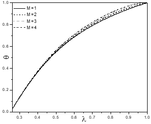
(b) θ(λ)
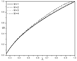
(c) S(λ)
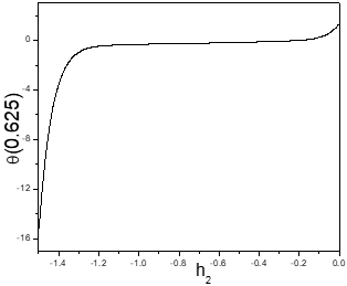
Figure 2. The h-curves for f(λ), θ(λ), S(λ) when Nr=1, Nt=0.5, Gr=10, R=1, Nb=1.0, Pr=1, A=1, Re=2, Le=1, Rd=1.5, M=2, Br=0.5, J=2.
In HAM, it is essential to see that the series solution converges. Also, the rate of convergence of approximation for the HAM solution mainly depend on the values of h. To find the admissible space of the auxiliary parameters, h-curves are drown for 16th-level of approximation and shown in figure 2. It is observed from this figure that the permissible range for h1, h2 and h3 are -0.6< h1< -0.05, -1.5< h2< -0 and -1.5 < h3< 0 respectively.
To obtain the optimal values of the auxiliary parameters, the following average residual errors [25] are computed and found that these errors are least at h1= - 0. 41, h2= -0.58 and h3= -1.12.
$E_{f, m}=\frac{1}{2 k} \sum_{i=-k}^{k}\left(N_{1}\left[\sum_{j=0}^{m} f_{j}(i \Delta t)\right]\right)^{2}$
$E_{\theta, m}=\frac{1}{2 k} \sum_{i=-k}^{k}\left(N_{2}\left[\sum_{j=0}^{m} \theta_{j}(i \Delta t)\right]\right)^{2}$
$E_{S, m}=\frac{1}{2 k} \sum_{i=-k}^{k}\left(N_{3}\left[\sum_{j=0}^{m} S_{j}(i \Delta t)\right]\right)^{2}$ (22)
where $\Delta t=\frac{1}{k}$ And k = 5. Also, for different values of m the series solutions are calculated and noticed that the series (16) converges in the total area of λ. Further, the graphs of the ratio
$\beta_{f}=\left|\frac{f_{m}(h)}{f_{m-1}(h)}\right|, \quad \beta_{\theta}=\left|\frac{\theta_{m}(h)}{\theta_{m-1}(h)}\right|, \quad \beta_{S}=\left|\frac{S_{m}(h)}{S_{m-1}(h)}\right|$ (23)
In contrast to the number of terms m in the homotopy series are calculated and observed that the series (17) converges to the exact solution.
The entropy generation volumetric rate of the nanofluid in concentric cylinders can be
expressed as
$S_{G}=\frac{K_{f}}{T_{a}^{2}}\left(\frac{\partial T}{\partial r}\right)^{2}+\frac{\mu}{T_{a}}\left[\left(\frac{\partial u}{\partial r}\right)^{2}-\frac{2 \mu}{r} \frac{\partial u}{\partial r}+\left(\frac{u}{r}\right)^{2}\right]$ $+\frac{\sigma B_{0}^{2} u^{2}}{T_{a}}+\frac{R u D}{\phi_{a}}\left(\frac{\partial \phi}{\partial r}\right)^{2}+\frac{R u D}{T_{a}}\left(\frac{\partial T}{\partial r}\right) \cdot\left(\frac{\partial \phi}{\partial r}\right)$ (24)
where Ru is the universal gas constant and D is the mass diffusivity through the fluid.
The entropy generation number Ns is the ratio of the volumetric entropy generation rate to the characteristic entropy generation rate according to Bejan [11]. Therefore, Ns is given by
$N s=\lambda^{3} \theta^{\prime 2}+\frac{B r}{\Omega_{1}}\left[\lambda^{2}\left(f^{\prime}\right)^{2}-2 \lambda f f^{\prime}+(f)^{2}\right]$ $+\phi_{1} \lambda^{3} S^{\prime 2}+\phi_{2} \lambda^{3} \theta^{\prime} S^{\prime}+\frac{J}{4 \Omega_{1}} \lambda^{2} f^{2}$ (25)
The dimensionless coefficients are $\phi_{1}$ and $\phi_{2}$ , called irreversibility distribution ratios which are related to diffusive irreversibility, given by
$\phi_{1}=\frac{R_{u} D}{K_{f} \cdot \Omega_{1}}\left(\frac{\Omega_{2}}{\Omega_{1}}\right) \Delta \phi$ , $\phi_{2}=\frac{R_{u} D}{K_{f} \cdot \Omega_{1}} \cdot \Delta \phi$ (26)
where $\Omega_{2}=\frac{\Delta \phi}{\phi_{a}}, \Omega_{1}=\frac{\Delta T}{T_{a}}$ are the concentration and temperature ratios, respectively and $\frac{K_{f} \Delta \mathrm{T}^{2}}{b^{2} T_{a}^{2}}$ is the characteristic entropy generation rate. The Eq.(25) can be expressed as
$N_{S}=N h+N v$ (27)
The entropy generation due to heat transfer irreversibility is denoted by the first term on the right hand side of the Eq.(27) and the entropy generation due to viscous dissipation is represented by second term of eq.(27). The ratio of the entropy generation (Ns) and the total entropy generation (Ns+Nv) is called Bejan number (Be). To understand the entropy generation mechanisms the Bejan number Be is specified. The Bejan number for this problem can be expressed as
$B e=\frac{N h}{N h+N v}$ (28)
In general, the limits of Bejan number is 0 to 1. Finally, the irreversibility due to viscous dissipation dominant represent by Be = 0, whereas Be = 1 represents the domination of heat transferirreversibility on Ns. It is clear that the heat transfer irreversibility is equal to viscous dissipation at Be=0.5.
The effects of chemical reaction, Joule heating, magnetic and Brinkman number on non-dimensional velocity, temperature and nanoparticle volume fraction, Bejan number Be and entropy generation Ns are presented graphically in figures 3-7. To study these effects of these parameters taking computations as Nr = 1, Nb =0.5, Gr = 10, Re = 2, Ω1 =0.1, Pr = 1, A = 1.0, Le = 1.0.
In order to assess the accuracy of HAM method, we have compared our results with the analytical solution of Sinha and Chaudhary (1966), as well as the spectral quasilinearization method (SQLM) of Srinivasacharya and Himabindu (2016) in the absence of Gr, A, Pr, Nt and Nb. The comparison in the above case is found to be in good agreement, as shown in Table 1.
Table 1. Comparison of HAM for the velocity against analytical and SQLM for Gr =0, A=0, Pr =0, Nt =0 and Nb = 0
|
λ |
Sinha & Chaudhury[29] Analytical solution |
Srinivasacharya &Himabindu [21] SQLM |
Present HAM |
|
0.25 |
0 |
0 |
0 |
|
0.2684 |
0.02453 |
0.024532 |
0.0245333 |
|
0.3216 |
0.09546 |
0.095462 |
0.0954667 |
|
0.4046 |
0.20613 |
0.206127 |
0.2061333 |
|
0.5091 |
0.34546 |
0.345462 |
0.3454677 |
|
0.625 |
0.5 |
0.5 |
0.5 |
|
0.7409 |
0.65453 |
0.654539 |
0.6545333 |
|
0.8454 |
0.793867 |
0.793863 |
0.7938673 |
|
0.9284 |
0.90453 |
0.904529 |
0.9045333 |
|
0.9816 |
0.97546 |
0.975468 |
0.9754676 |
|
1 |
1 |
1 |
1 |
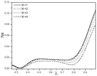
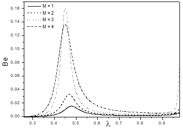
The variation of velocity component, temperature, nanoparticle concentration, Ns and Be with magnetic parameter M are presented in figure (3). It is noticed from figure (3a) that, the dimensionless velocity is decreasing with an enhancement in the magnetic parameter M. Since the transverse magnetic field which is applied normal to the direction of flow gives a resistive force known as Lorentz force. This Lorentz force resists the flow of a nanofluid therefore the velocity decreases. Figure (3b) reveals that, the dimensionless temperature θ(λ) is increasing with a rise in the magnetic parameter M. There is an increase in the nanoparticle concentration S(λ) with an increase in the magnetic parameter M as depicted in figure (3c). Figure (3d) shows that the entropy generation decays with a growth in the magnetic parameter M. It is clear from figure (3e) that Be is increasing with an enhancement in the value of M. The maximal value of Be is observed at the center of the annular region due to more contribution of heat transfer irreversibility on entropy generation. It is observed that the fluid friction dominates near the cylinders.
(a) f(λ)
(b) θ(λ)
(c) S(λ)
(d) Ns
(e) Be
Figure 3. Effect of Magnetic parameter on velocity f(λ), temperature θ(λ), nanoparticle concentration S(λ), Entropy generation Ns and Bejan number Be.
(a) f(λ)
(b) θ(λ)
(c) S(λ)
(d) Ns
(e) Be
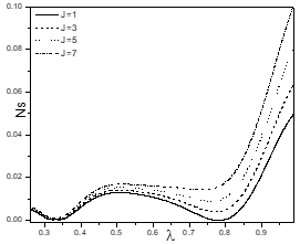
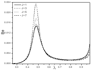
Figure 4. Effect of Joule heating parameter on velocity f(λ), temperature θ(λ), nanoparticle concentration S(λ), Entropy generation Ns and Bejan number Be.
The influence of the Joule heating parameter on f(λ), θ(λ), nanoparticle concentration S(λ), Ns and Be is shown in figure (4). The dimensionless velocity f(λ) rises with a rise in the Joule heating parameter J as shown in figure (4a). Figure (4b) reveals that θ(λ) rises with a rise in the Joule heating parameter J. As the Joule heating parameter J increases in the fluid flow, some of the kinetic energy is converted into the heat and as a result temperature of the body increases. From figure (4c), it is noticed that the nanoparticle concentration S(λ) decays with a growth in the Joule heating parameter J. Figure (4d) shows that increase in the Joule heating parameter causes an increase in the entropy generation. An increase in the Joule heating parameter J, the Bejan number increases near the inner cylinder and away from the inner cylinder the trend is reversed due to more contribution of heat transfer irreversibility on Ns as presented in figure (4e). It is observed that the fluid friction dominates near the cylinders and heat transfer irreversibility dominates around the center of an annulus.
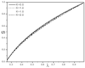
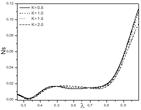
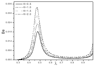
Figure (5) displays the impact of the chemical reaction K on velocity in flow direction, temperature, nanoparticle concentration, entropy generation and Bejan number. Figure (5a) reveals that the velocity is increasing with an increase in the chemical reaction parameter K. The effect of the chemical reaction K on the non-dimensional the temperature θ(λ) is presented in figure(5b). From this figure, it is observed that θ(λ) decays with an enhancement in the chemical reaction parameter K. The influence of K is to reduce the temperature extremely in the flow field. Figure (5c) depicts the variation of nanoparticle concentration with K. The nanoparticle concentration S(λ) decreases with a rise in the chemical reaction parameter K. Figure (5d) shows that the entropy generation decreases near the cylinders, while away from the cylinders the trend is reversed due to high temperature gradient in this region, as an increase in the chemical reaction parameter K. It is clear from figure (5e) that Be increasing with an enhancement in the value of the chemical reaction K. The maximal value of Bejan number is noticed at the center of an annular region due to more contribution of heat transfer irreversibility on Ns and it is noticed that the fluid friction dominated near the cylinders.
(a) f(λ)
(b) θ(λ)
(c) S(λ)
(d) Ns
(e) Be
Figure 5. Effect of Chemical reaction parameter on velocity f(λ), temperature θ(λ), nanoparticle concentration S(λ), Entropy generation Ns and Bejan number Be.
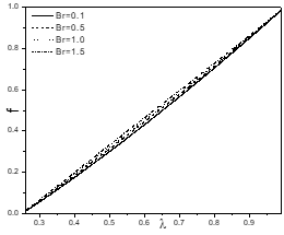
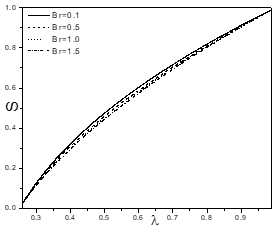
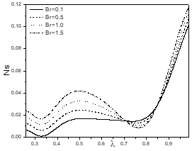
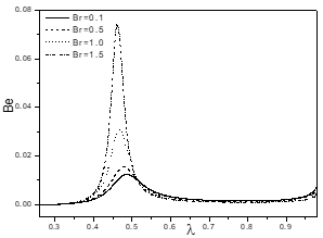
The impact of the Brinkman number Br on f(λ), θ(λ) S(λ), Ns and Be is depicted in figure (6). The dimensionless velocity f(λ) rises with a rise in Brinkman number Br as shown in figure (6a). Figure (6b) reveals that θ(λ) rises with a rise in Br. From figure (6c) it is noticed that nanoparticle concentration S(λ) decays with a growth in Brinkman number Br. Figure (6d) shows that an increase in Br, causes an increase in the entropy generation. As Br increases, an increase in Bejan number is observed near the inner cylinder, while away from the inner cylinder the trend is reversed due to more contribution of the heat transfer irreversibility on entropy generation and Be is decreasing near the outer cylinder as presented in figure (6e). It is noticed that the fluid friction dominated near the end points of cylinders and heat transfer irreversibility dominated around the center of an annulus.
(a) f(λ)
(b) θ(λ)
(c) S(λ)
(d) Ns
(e) Be
Figure 6. Effect of Brinkman number on velocity f(λ), temperature θ(λ), nanoparticle concentration S(λ), Entropy generation Ns and Bejan number Be.
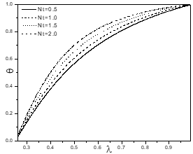
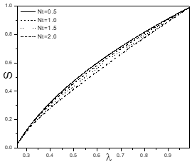
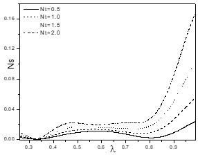
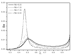
Figure (7) shows the effect of thermophoresis parameter Nt on velocity in flow direction f(λ), temperature θ(λ), nanoparticle concentration S(λ), Bejan number Be and entropy generation Ns. The velocity in flow direction f(λ) increases with an enhancement in the thermophoresis parameter Nt as shown in figure (7a). Figure (7b) reveals that, the dimensionless temperature θ(λ) increases with an increase in the thermophoresis parameter Nt. Increase in the thermophoresis parameter Nt leads to increase the effective-conductivity, hence the nanoparticle concentration S(λ) is decreasing, it is recognized from figure (7c). It is noticed from figure (7d) that the entropy generation is increasing with an enhancement in the thermophoresis parameter Nt. As the thermophoresis parameter Nt increases, an increase in the Bejan number is observed near the inner cylinder, while away from the cylinder the trend is reversed due to more contribution of heat transfer irreversibility on Ns and Be is decreasing near the outer cylinder as presented in figure (7e).
(a) f(λ)
(b) θ(λ)
(c) S(λ)
(d) Ns
(e) Be
Figure 7. Effect of Thermophoresis parameter on velocity f(λ), temperature θ(λ), nanoparticle concentration S(λ), Entropy generation Ns and Bejan number Be
In this article, the entropy generation due to a chemically reacting nanofluid in mixed convective flow between two concentric cylinders is analyzed by considering magnetic, Joule heating and thermophoresis parameter effects. The non-dimensional nonlinear equations are solved by the HAM. The main observations are summarized below
• As the Joule heating parameter increases, the dimensionless temperature, velocity and entropy generation increase, but the nanoparticle concentration decreases.
• The dimensionless velocity and Bejan number are increasing, whereas the temperature, nanoparticle concentration and entropy generation are decrease with a rise in the chemical reaction K.
• As Brinkman number increases, the velocity, temperature, entropy generation increase, but the nanoparticle concentration decreases.
• As the thermophoresis parameter increases, the velocity, temperature, entropy generation increase, but the nanoparticle concentration decreases.
• The maximum values of Be are observed at the center of an annulus due to more contribution of heat transfer irreversibility on Ns and minimum value is near the cylinders, due to more contribution of fluid friction irreversibility on Ns with an enhancement in K, M, Br, J and Nt.
|
A |
Constant pressure gradient |
|
A |
Radius of the inner cylinder |
|
B |
Radius of the outer cylinder |
|
B0 |
Magnetic field |
|
Be |
Bejan number |
|
Br |
Brinkman number |
|
Cp |
Specific heat capacity |
|
D |
Mass diffusivity |
|
DB |
Brownian diffusion coefficient |
|
DT |
Thermophoresis diffusion coefficient |
|
g |
Acceleration due to gravity |
|
Gr |
Grashof number |
|
J |
Joule heating parameter |
|
Kf |
Coefficient of thermal conductivity |
|
K |
Chemical reaction parameter |
|
k1 |
Rate of chemical reaction |
|
Le |
Lewis number |
|
M |
Magnetic parameter |
|
Nb |
Brownian motion parameter |
|
Nr |
Buoyancy ratio |
|
Ns |
Entropy generation |
|
Nt |
Thermophoresis parameter |
|
Nh |
Entropy generation due to heat transfer |
|
Nv |
Entropy generation due to viscous dissipation |
|
p* |
Pressure |
|
Pr |
Prandtl number |
|
Re |
Reynolds’s number |
|
Ru |
Universal gas constant |
|
SG |
Entropy generation volumetric rate |
|
Tm |
Mean fluid temperature |
|
T |
Temperature |
|
u |
Velocity |
|
Greek Symbols |
|
|
ϕ |
Nanoparticle concentration |
|
m |
Viscosity coefficient |
|
r |
Density of the fluid |
|
s |
Electrical conductivity |
|
a |
Effective thermal diffusivity |
|
bT |
Coefficients of thermal expansion |
|
Subscripts |
|
|
‘ Differentiation with respect to λ |
|
[1] Choi S.U.S., Eastman J.A. (1995). Enhancing thermal conductivity of fluids with nanoparticles, ASME Fed, Vol. 231, No. 1, pp. 99-105.
[2] Sheikhzadeh G.A., Teimouri H., Mahmoodi M. (2013). Numerical study of mixed convection of nanofluid in a concentric annulus with rotating inner cylinder, Trans. Phenom. Nano Micro Scales, Vol. 1, No. 1, pp. 26-36.
[3] Togun H., Abdulrazzaq T., Kazi S.N., Badarudin A., Kadhum A.A.H., Sadeghinezhad E. (2014). A review of studies on forced, natural and mixed heat transfer to fluid and nanofluid flow in an annular passage, Renewable and Sustainable Energy Reviews, Vol. 39, pp. 835-856.
[4] Nandkeolyar R., Motsa S.S., Sibanda P. (2013). Viscous and joule heating in the stagnation point nanofluid flow through a stretching sheet with homogenous–heterogeneous reactions and nonlinear convection, Journal of Nanotechnology in Engineering and Medicine, Vol. 4, pp. 1-9.
[5] Zhang J.K., Li B.W., Chen Y.Y. (2015). The joule heating effects on natural convection of participating magnetohydrodynamics under different levels of thermal radiation in a cavity, Journal of Heat Transfer, Vol. 137, pp. 1–10.
[6] Hayat T., Shafique M., Tanveer A., Alsaedi A. (2016). Hall and ion slip effects on peristaltic flow of Jeffrey nanofluid with Joule heating, Journal of Magnetism and Magnetic Materials, Vol. 407, pp. 51-59.
[7] Dulal P., Babulal T. (2011). Combined effects of Joule heating and chemical reaction on unsteady magnetohydrodynamics mixed convection of a viscous dissipating fluid over a vertical plate in porous media with thermal radiation, Mathematical and Computer Modelling, Vol. 54.
[8] Mridulkumar G. (2015). Effects of chemical reaction on MHD boundary layer flow over an exponentially stretching sheet with joule heating and thermal radiation, International Research Journal of Engineering and Technology, Vol. 2, No. 09, pp. 768-773.
[9] Poulomi De., Hiranmoy M., Uttamkumar B. (2015). Effects of mixed convective flow of a nanofluid with internal heat generation, thermal radiation and chemical reaction, Journal of Nanofluids, Vol. 4, No. 3, pp. 375-384.
[10] Bejan A. (1995). Entropy Generation Minimization, CRC Press, Boca Raton, New York.
[11] Bejan A. (1996). Entropy Generation through Heat and Fluid Flow, Wiley, CRC Press, New York.
[12] Gyftopoulos E.P., Beretta G.P. (1993). Studied the entropy generation rate in a chemically reacting system, J.of Egy Resources Tech., Vol. 115. pp. 208-212.
[13] Miranda E.N. (2010). Entropy generation in a chemical reaction, Eur. J. Phys., Vol. 31, pp. 267-277.
[14] Imen C., Nejib H., Ammar B.B. (2014). Entropy generation analysis of a chemical reaction process, J. of Heat and Transfer, Vol. 136.
[15] Govindaraju M., Vishnu Ganesh N., Ganga B., Abdulakeem, A.K. (2015). Entropy generation analysis of magnetohydrodynamic flow of a nanofluid over a stretching sheet, Journal of the Egyptian Mathematical Society, Vol. 23, pp. 429-434.
[16] Rashidi M.M., Bhatti M.M., Munawwar A.A., Ali M.E.S. (2016). Entropy generation on MHD blood flow of nanofluid due to peristaltic waves, Entropy, Vol. 18, pp. 1-10.
[17] Fersadou I., Kahalerras H., El Ganaoui M. (2015). MHD mixed convection and entropy generation of a nanofluid in a vertical porous channel, Computers and Fluids, Vol. 121, pp. 164-179.
[18] Omid M., Mahmud S., Saeed Z.H. (2012). Analysis of entropy generation between co-rotating cylinders using nanofluids, Energy, Vol. 44, pp. 438-446.
[19] Omid M., Ali K., Clement K., AlNimr M.A., Ioan P., Sahin A.Z., Somchai W. (2013). A review of entropy generation in nanofluid flow, International Journal of Heat and Mass Transfer, Vol. 65, pp. 514-532.
[20] Mohammad D., Nemat D., Mohammad R.H.N. (2014). Numerical analysis of entropy generation in nanofluid flow over a transparent plate in porous medium in presence of solar radiation, viscous dissipation and variable magnetic field, Journal of Mechanical Science and Technology, Vol. 28, No. 5, pp. 1819-1831.
[21] Srinivasacharya D., Himabindu K. (2016). Entropy generation due to micropolar fluid flow between concentric cylinders with slip and convective boundary conditions, Ain Shams Engineering Journal, in press.
[22] Liao S.J. (2003). Beyond Perturbation, Introduction to Homotopy Analysis Method, Chapman and Hall/CRC Press, Boca Raton.
[23] Buongiorno J. (2006). Convective transport in nanofluids, ASME J Heat Transfer, Vol. 128, pp. 240-250.
[24] Liao S.J. (2004). On the homotopy analysis method for nonlinear problems, Appl Math Comput, Vol. 147, No. 2, pp. 499-513.
[25] Liao S.J. (2010). An optimal homotopy-analysis approach for strongly nonlinear differential equations, Commun Nonlinear Sci. Numer Simul, Vol. 15, pp. 200-316.
[26] Liao S.J. (2013). Advances in the Homotopic Analysis Method, World Scientific Publishing Company, Singapore.
[27] Sinha K.D. Chaudhary R.C. (1966). Viscous incompressible flow between two coaxial rotating porous cylinders, Proc Nat Inst Sci., Vol. 32, pp. 81-88.