OPEN ACCESS
In this paper, we investigate the effect of variation in thermal conductivity on several transient heat transfer problems with the lattice Boltzmann method (LBM). First, benchmark problems involving radiation and/or conduction with constant thermal conductivity are simulated. Then we consider the case of variable thermal conductivity with temperature in solving 2D coupled conduction-radiation heat transfer problem and natural convection in differentially heated enclosure. Both the energy equation and the radiative transfer equation (RTE) were solved using exclusively the lattice Boltzmann method. Good agreement with available data in literature was obtained.
LBM, RTE, variable thermal conductivity, conduction, natural convection
Variable thermal conductivity heat transfer occurs in many engineering applications. Examples of combined conduction and radiation problems in which the change of temperature and hence the variation of thermal conductivity are large, includes heat transfer in furnaces, boilers, porous burners or even volumetric solar receivers [1]. In all those heat transfer problems, temperature varies over a wide range. Thus the assumption of constant thermal conductivity provides less accurate results [2, 3].
The Lattice Boltzmann Method (LBM) has achieved considerable success in simulating various transport phenomena in last two decades [4]. It’s a mesoscopic approach based on the kinetic theory and the integro- differential Boltzmann equation [5]. Its main asset is its simple algebraic manipulation, its easy solution procedure and implementation of boundary conditions, together with its ability of dealing with complex fluids [6], phase change phenomenon [7] and nanofluids [8], etc. In order to benefit from some known LBM advantages and to correctly deal with variable thermal conductivity problems, some refinements has to be done. Knowing that when solving such problems, the relaxation time is important, one have to be careful in implementing the correct expression of the relaxation time expression.
Talukdar and Mishra [9] investigated the effect of variable thermal conductivity on transient conduction and radiation heat transfer in a planar medium with the lattice Boltzmann method for solution of the energy equation and with the discrete transfer method (DTM) for the radiative information.To account for the variation in thermal conductivity with temperature, the authors used a time linearization technique based on updated values of temperature calculated with data available from a previous iteration.
Mishra et al. [10] solved combined conduction-radiation heat transfer problems by means of the lattice Boltzmann method and investigated the variation effect of thermal conductivity as well as refractive index on temperature distribution at steady state. To deal with variation in thermal conductivity a modified relaxation time expression was used.
Hazi and Markus [11] proposed in their work to use the lattice Boltzmann method to simulate classical heat transfer problems of supercritical fluids. They considered a supercritical fluid layer between two plates and investigated the piston effect by simulating heat transfer in a supercritical fluid layer near the critical point. To account for the variable part of the thermal conductivity, they considered a different expression of the equilibrium distribution function by adding an extra term to this function.
In this paper, we apply the idea proposed by [11] to correctly treat variation in thermal conductivity by a modified expression of the equilibrium distribution function used in collision step of the lattice Boltzmann method. First benchmark problems involving radiation and/or conduction with constant thermal conductivity are simulated. Then we consider the case of variable thermal conductivity with temperature in solving coupled conduction-radiation 2D heat transfer problem and natural convection in 2D differentially heated enclosure.
The paper is organized as follows. In section 2, we present the different cases of benchmark problems solved by means of the modified thermal lattice Boltzmann method. The formulation of solving radiative transfer equation by lattice Boltzmann method is presented next. In section 3, the benchmark problems are presented with detailed boundary conditions. Simulation results are also presented in this section. Section 4 concludes the paper.
We consider the following cases of benchmark problems:
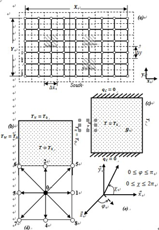
-Case 1: In this case, the boundaries of the 2-D rectangular medium (Figure 1a) are the known radiation source and temperature of the absorbing, emitting and scattering medium is unknown. Further, heat fluxes along the enclosure boundaries are also unknown. Enclosure boundaries can be at arbitrary temperatures. This case belongs to a benchmark radiative equilibrium problem in which, in comparison to radiation, conduction and convection modes are insignificant.
-Case 2: Initially at t = 0, the 2-D rectangular system is at temperature T0 and for time t > 0, the south boundary is raised and maintained at a higher temperature Ts = 2 T0 (Figure 1b). Uniform volumetric heat generation source may be present in the enclosure. In this case, along with radiation, effect of conduction is also important. This is a benchmark 2-D conduction-radiation problem that has been investigated by many researchers. All four boundaries are diffusing and gray.
-Case 3: For this case, we adopt a variable thermal conductivity, l which is a linear function of temperature
$\lambda=\lambda_{0}+\gamma\left(T-T_{r f}\right)$ (1)
where l0 is the thermal conductivity at reference temperature Tref, g' is the coefficient of thermal conductivity variation. The heat transfer problems under consideration for the variation of thermal conductivity with temperature, includes transient conduction-radiation in square enclosure and heat transfer by natural convection with heat generation rate.
It is to be noted that to ensure that the flow is fully in the incompressible regime, Ma should satisfy incompressible limit. Given that, the characteristic velocity in thermal convective flows which is defined as
$U=\sqrt{\propto g \Delta T L}=\frac{\sqrt{R a}}{\operatorname{Pr}} \frac{v}{L}$ (2)
The Mach number based on U should be small in order to comply with incompressible approximation of the flow and also the stability criterion on the viscosity ν [12].
Suppose that U< cs Ma for some critical Mach number Ma (usually Ma<0.3), and cs is the speed of sound, then the viscosity n has the following upper bound given by
$\sqrt{3 R a} v \prec M a L \sqrt{\mathrm{Pr}}$ (3)
where the length L is measured in the lattice unit Δx=1
1.1 LBM for variable thermal conductivity
For computation of temperature field, the governing lattice Boltzmann equation is given by [13]
$\begin{aligned} f_{i}\left(\vec{r}+\vec{e}_{i} \Delta t, t+\Delta t\right) &=f_{i}(\vec{r}, t)-\frac{\Delta t}{\tau_{t}}\left[f_{i}(\vec{r}, t)-f_{i}^{e q}(\vec{r}, t)\right] \\ i &=0,1,2, \ldots, b \end{aligned}$ (4)
where fi is the particle distribution function, $\vec{e}_{i}$ is the microscopic velocity, is the relaxation time and $f_{i}^{\mathrm{cq}}$ is the equilibrium distribution function.
For the D2Q9 lattice (Figure 1b) used in the present work, the relaxation time is computed from [13
$\tau_{t}=\frac{3 \alpha}{\left|\vec{e}_{i}\right|^{2}}+\frac{\Delta t}{2}$ (5)
For the case where the conductivity is a function of temperature, the equilibrium distribution function needs to be modified as below [11]
$f_{i}^{e q}=w_{i}\left[T+\frac{1}{c_{s}^{2}} T \vec{e}_{i} . \vec{u}-\frac{D}{c_{s}^{2}} \vec{e}_{i} . \vec{\nabla} T\right]$ (6)
where D is the variable part of the thermal diffusivity, which can be set as a function of the position, time temperature and any of the dependent flow parameter.
Figure 1. (a) Geometry and the coordinates of the problem under consideration, (b) physical problem with Dirichlet boundary conditions, (c) physical model for natural convection (d) D2Q9 lattice structure (e) coordinate used in solving radiative transfer equation
2.2 LBM for density and velocity field
For computation of density and velocity field, the governing lattice Boltzmann equation is given by [13]
$\begin{aligned} g_{i}\left(\vec{r}+\vec{e}_{i} \Delta t, t+\Delta t\right) &=g_{i}(\vec{r}, t)-\frac{\Delta t}{\tau_{v}}\left[g_{i}(\vec{r}, t)-g_{i}^{e q}(\vec{r}, t)\right]+\Delta t \times F \\ i &=0,1,2, \ldots, b \end{aligned}$ (7)
where gi is the particle distribution function, is the microscopic velocity, tn is the relaxation time, is the equilibrium distribution function, and F is the external force term.
For the D2Q9 lattice (Figure 1d) used in the present work,the relaxation time tn is computed from [13]
$\tau_{t}=\frac{3 v}{\left|\vec{e}_{i}\right|^{2}}+\frac{\Delta t}{2}$ (8)
with Prandtl number Pr and Rayleigh number Ra known,the kinetic viscosity v appearing in Equation (8) is computed from simultaneously solving the following two equations:
$P r=\frac{v}{\alpha}$ (9)
$R a=\frac{\beta_{t} g\left(T_{h}-T_{c}\right) H^{3}}{\alpha v}$ (10)
where a is the thermal diffusivity, b is the coefficient of thermal expansion, g is the acceleration due to the gravity, This the hot wall temperature, Tc is the cold wall temperature,and H is the height and width of the cavity.The equilibrium function for the density distribution function is given as
$\begin{aligned} g_{i}^{e q} &=w_{i}\left[1+3\left(\vec{e}_{i} . \vec{u}\right)+\frac{9}{2}\left(\vec{e}_{i} . \vec{u}\right)-\frac{3}{2} \vec{u}^{2}\right] \\ 0 & \leq i \leq 8 \end{aligned}$ (11)
ei the lattice speed for the D2Q9 model are given by
$\vec{e}_{i}=\left\{\begin{array}{rlr}{0} & {i=0} \\ {C\{\cos [(i-1) \pi / 2], \sin [(i-1) \pi / 2]\}} & {1 \leq i \leq 4} \\ {\sqrt{2} C\{\cos [(i-5) \pi / 2+\pi / 4], \sin [(i-5) \pi / 2+\pi / 4]\}} & {5 \leq i \leq 8}\end{array}\right.$
For the D2Q9 model the weights are given by
$w_{i}=\left\{\begin{array}{ll}{4 / 9} & {i=0} \\ {1 / 9} & {1 \leq i \leq 4} \\ {1 / 36} & {5 \leq i \leq 8}\end{array}\right.$ (12)
2.3 LBM for thermal field
In the presence of volumetric radiation, for a 2-Drectangular enclosure containing a radiating-conducting medium, the governing energy equation, reads
$\rho C_{p} \frac{\partial T}{\partial t}=\frac{\partial}{\partial x}\left(\lambda \frac{\partial T}{\partial x}\right)+\frac{\partial}{\partial y}\left(\lambda \frac{\partial T}{\partial y}\right)-\vec{\nabla} \cdot \vec{q}_{R}+g$ (13)
where $\rho$ and $C_{p}$ are the density and the specific heat,respectively. The last term in energy equation stand for the radiative source term, which is the divergence of radiative heat flux
$\vec{\nabla} \cdot \vec{q}_{R}=k_{a}\left[4 \pi\left(\frac{\sigma T^{4}}{\pi}\right)-G\right]$ (14)
where ka, T and G, are the absorption coefficient, the temperature and the volumetric incident radiation, respectively. The expression of the volumetric radiation G is given in the next section.
Substituting for $\lambda$ from Equation (1) into Equation (13),we get
$\rho C_{p} \frac{\partial T}{\partial t}=\left[\lambda_{0}+\gamma^{\prime}\left(T-T_{r e f}\right)\right]\left(\frac{\partial^{2} T}{\partial x^{2}}+\frac{\partial^{2} T}{\partial y^{2}}\right)+\gamma^{\prime}\left[\left(\frac{\partial T}{\partial x}\right)^{2}+\left(\frac{\partial T}{\partial y}\right)^{2}\right]-\vec{\nabla} \cdot \vec{q}_{R}+g$ (15)
For generality, we use dimensionless parameters, viz.distance $r^{+}$, time , temperature , conduction-radiation parameter N, incident radiation G+, radiative heat flux ,heat generation $g^{+}$ and variable part of thermal conductivity $\gamma$ defined as:
$r^{+}=\frac{r}{L}, \xi=\alpha \beta^{2} t, \theta=\frac{T}{T_{r e f}}$$N=\frac{\lambda_{0} \beta}{4 \sigma T_{r e f}^{3}}, G^{+}=\frac{G}{\left(\sigma T_{r e f}^{4} / \pi\right)}$$\psi_{R}=\frac{q_{R}}{\sigma T_{r e f}^{4}}, I^{+}=\frac{I}{\left(\sigma T_{r e f}^{4} / \pi\right)}$$g^{+}=\frac{g}{\alpha T_{r e f} \beta^{2}}, \gamma=\gamma^{\prime} T_{r e f} N$ (16)
In dimensionless form, Equation (14) becomes
$\frac{\partial \theta}{\partial \xi}=\frac{1}{\tau^{2}}[1+\gamma(\theta-1)]\left(\frac{\partial^{2} \theta}{\partial x^{+2}}+\frac{\partial^{2} \theta}{\partial y^{+2}}\right)+\frac{\gamma}{\tau^{2}}\left[\left(\frac{\partial \theta}{\partial x^{+}}\right)^{2}+\left(\frac{\partial \theta}{\partial y^{+}}\right)^{2}\right]-\frac{1}{N} \vec{\nabla} \cdot \vec{\psi}_{R}+g^{+}$ (17)
where
$\vec{\nabla} \cdot \vec{\psi}_{R}=\beta(1-\omega)\left[\theta^{4}-\frac{G^{+}}{4 \pi}\right]$ (18)
In the LBM, the equivalent form of the energy equation (Equation (13)) is given by [14-16]
$\begin{aligned} f_{i}\left(\vec{r}+\vec{e}_{i} \Delta t, t+\Delta t\right)=& f_{i}(\vec{r}, t)-\frac{\Delta t}{\tau_{t}}\left[f_{i}(\vec{r}, t)-f_{i}^{e q}(\vec{r}, t)\right] \\ &-\left(\frac{\Delta t}{\rho C_{p}}\right) w_{g i} \vec{\nabla} \cdot \vec{q}_{R}+\Delta t w_{i} g \\ i &=0,1,2, \ldots, b \end{aligned}$ (19)
Once the values of fi over all directions are known, in a conduction-radiation problem, temperature T is calculated from the following
$T(\vec{r}, t)=\sum_{i=0}^{b} f_{i}(\vec{r}, t)$ (20)
In dimensionless form, Equation (19) becomes
$\begin{aligned} f_{i}^{+}\left(\vec{r}^{+}+\vec{e}_{i}^{+} \Delta \xi, \xi+\Delta \xi\right) &=f_{i}^{+}\left(\vec{r}^{+}, \xi\right) \\ &-\frac{\Delta \xi}{\tau_{t}^{+}}\left[f_{i}^{+}\left(\vec{r}^{+}, \xi\right)-f_{i}^{+e q}\left(\vec{r}^{+}, \xi\right)\right] \\ &-\left(\frac{\Delta \xi}{N}\right) w_{g i} \vec{\nabla} \cdot \vec{\psi}_{R}+\Delta \xi w_{i} g^{+} \\ i &=0,1,2, \ldots, b \end{aligned}$ (21)
The dimensionless relaxation time $\tau_{t}^{+}$ is given by
$\tau_{t}^{+}=\frac{3}{\left|\frac{\Delta r^{+}}{\Delta \xi}\right|^{2}}+\frac{\Delta \xi}{2}$ (22)
where $\frac{\Delta r^{+}}{\Delta \xi}$, is the dimensionless velocity.The new temperature field is obtained with summing the non-dimensional distributions function as follow
$\theta\left(\vec{r}^{+}, \xi\right)=\sum_{i=0}^{8} f_{i}^{+}\left(\vec{r}^{+}, \xi\right)$ (23)
2.4 LBM for radiative transfer equation The LBM formulation for the radiative transfer equation is given as follows [17]
$\frac{\partial I}{\partial s}+\hat{s} \times \nabla I=-\beta I+k_{a} I_{b}+\frac{\sigma_{S}}{4 \pi} \int_{4 \pi} I p\left(\Omega, \Omega^{\prime}\right)$ (24)
With the assumption of isotropic scattering, $p\left(Q, \Omega^{\prime}\right)=1$,Equation (24) can be written as
$\frac{d I}{\partial s}+\hat{s} \times \nabla I=\beta\left(\frac{G}{4 \pi}-I\right)$ (25)
The transient equation for the discrete direction is
$\frac{D_{i} I_{i}}{D t}=e_{i} \beta\left(\frac{G}{4 \pi}-I\right) i=1,2, \ldots, M$ (26)
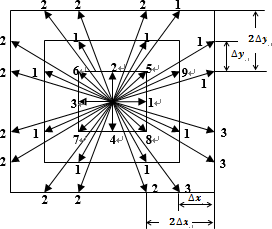
M is the total number of discrete lattice direction. For the D2Q8, D2Q16 and D2Q32, lattices shown in (Figure 2) M=8,16 and 32 respectively. Equation (26), in lattice Boltzmann form is as below [17]
$I_{i}\left(\vec{x}_{n}+\vec{e}_{i} \Delta t, t+\Delta t\right)=I_{i}\left(\vec{x}_{n}, t\right)+\Delta t e_{i} \beta\left(\frac{G}{4 \pi}-I\right)$ (27)
Assuming a relaxation time $\tau_{i}=\frac{1}{e_{i} \beta}$, Equation (27) is written as follows
$\begin{aligned} I_{i}\left(\vec{x}_{n}+\vec{e}_{i} \Delta t, t+\Delta t\right)=& I_{i}\left(\vec{x}_{n}, t\right) \\ &+\frac{\Delta t}{\tau_{i}}\left[I_{i}^{e q}\left(\vec{x}_{n}, t\right)-I_{i}\left(\vec{x}_{n}, t\right)\right] \end{aligned}$ (28)
The equilibrium distribution function in Equation (28) is given by [17]
$I_{i}^{e q}=\sum_{i=1}^{N_{v}} I_{i} w_{g i}$ (29)
$\mathcal{W}_{g i}=\left(\frac{1}{4 \pi}\right) \int_{0}^{\pi} \sin \varphi d \varphi \int_{\chi_{i}-\left(\frac{\Delta \chi_{i}}{2}\right)}^{\chi_{i}+\left(\frac{\Delta \chi_{i}}{2}\right)} d \chi=\frac{\Delta \chi_{i}}{2 \pi}$ (30)
The radiative heat flux in x- and y-direction, are given by [18]
$q_{x}=\sum_{i=1}^{N_{v}} I_{i} w_{x i} \quad q_{y}=\sum_{i=1}^{N_{v}} I_{i} w_{y i}$ (31)
Figure 2. Schematic of the lattices D2Q8: 1–8, D2Q16: 1–16 and D2Q32: 1–32 directions used for calculation of radiative information [18]
The corresponding weights in Equation (31) are given by [18]
$w_{x i}=\int_{0}^{\pi} \sin ^{2} \varphi d \varphi \int_{\chi_{i}-\left(\frac{\Delta \chi_{i}}{2}\right)}^{\chi_{i}+\left(\frac{\Delta \chi_{i}}{2}\right)}$$\cos \chi d \chi=\pi \cos \chi_{i} \sin \left(\frac{\Delta \chi_{i}}{2}\right)$
$w_{y i}=\int_{0}^{\pi} \sin ^{2} \varphi d \varphi \int_{\chi_{i}-\left(\frac{\Delta \chi_{i}}{2}\right)}^{\chi_{i}+\left(\frac{\Delta \chi_{i}}{2}\right)}$$\sin \chi d \chi=\pi \sin \chi_{i} \sin \left(\frac{\Delta \chi_{i}}{2}\right)$ (32)
3.1 Radiative equilibrium
When dealing with the first case (radiative equilibrium),the grid mesh used is (101 101) [17]. For this case we assume that the south boundary is raised at a temperature Ts and the other three boundaries are cold and black. We define the dimensionless heat flux and emissive power, respectively as:
$\psi_{R}=\frac{q_{R y}}{\sigma T_{s}^{4}} \quad \phi=\frac{\sigma T^{4}}{\sigma T_{s}^{4}}$ (33)
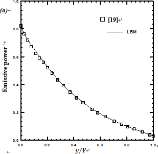
Dimensionless centerline emissive power distribution for two values of the extinction coefficient,$\beta=3.0$ and $\beta=5.0$ have been compared in Figure 3(a)-(b), respectively.Results of the LBM and FVM [19] are in very good agreements.
Figure 3. Comparison of the centerline $\left(\frac{x}{X}=0.5, y\right)$ emissive power for (a) $\beta=3.0,$ (b) $\beta=5.0$
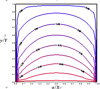
In Figure 4, results of the dimensionless heat flux y R obtained from the LBM, is compared with that of the FVM [19]. In this figure, comparison has been made for, $\beta=3.0$ and $\beta=5.0$ . It is seen that for all the cases, the LBM and the FVM results are in good agreements. In Figure 5, the distribution of the dimensionless temperature in the square enclosure for $\beta=3.0$ is highlighted.
Figure 4. Comparison of radiative heat flux $\psi_{R}$ along the bottom (hot) wall for different values of the extinction coefficient $\beta$
Figure 5. Distribution of the dimensionless temperature in the square enclosure for $\beta=3.0$
3.2 Combined conduction-radiation
Table 1. Comparison of steady-state centerline temperature at three locations in a black square enclosure $\beta=1.0, \omega=0.0$
|
N |
Centerline q at y Y = |
Ref.
[13] |
Ref.
[20] |
Ref.
[21] |
LBM- LBM (Present) |
|
1.0 |
0.3 |
0.733 |
0.737 |
0.737 |
0.737 |
|
|
0.5 |
0.630 |
0.630 |
0.630 |
0.630 |
|
|
0.7 |
0.560 |
0.560 |
0.564 |
0.564 |
|
0.1 |
0.3 |
0.760 |
0.763 |
0.759 |
0.759 |
|
|
0.5 |
0.663 |
0.661 |
0.663 |
0.662 |
|
|
0.7 |
0.590 |
0.589 |
0.594 |
0.596 |
|
0.01 |
0.3 |
0.791 |
0.807 |
0.789 |
0.806 |
|
|
0.5 |
0.725 |
0.726 |
0.725 |
0.723 |
|
|
0.7 |
0.663 |
0.653 |
0.666 |
0.666 |
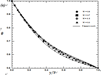
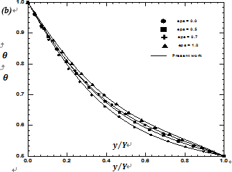
To validate our codes we consider at first, the case of constant thermal conductivity $\gamma=0.0$. We provide steady-state results for dimensionless temperature with those available in References [13, 20, 21]. With $\beta=1.0$ and $\omega=0.0$. This validation has been shown for three values of the conduction-radiation parameter N. Centerline temperature $\theta$ distribution has been compared at three locations along the centerline (Table 1). Next in Figure 6(a) and 6(b), the effect of scattering albedo $\omega$ and extinction coefficient, on dimensionless steady-state temperature distribution along the centerline $\left(\frac{x}{X}=0.5, y\right)$ are shown, respectively. After,Figure 7(a)-(d) highlights the effect of conduction-radiation N and hot wall emissivity .
Figure 6. Comparison of the steady state centerline temperature
$\theta=T / T_{\text {ref}}$ for different parameter with those obtained by [19] (a) $N=0.1, \beta=1.0, \varepsilon_{S}=1.0$ and different values of scattering albedo , (b) $N=0.1, \omega=0.0, \beta=1.0$ and different values of hot wall emissivity $\varepsilon_{S}$
With fixed values of the extinction coefficient and conduction-radiation parameter, N=0.1, the increase in makes the medium scatter more and tend to the case of the conduction phenomenon domination [Figure 6(a)]. In Figure 6(b), effect of hot wall emissivity is provided.
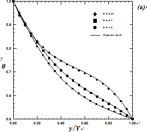
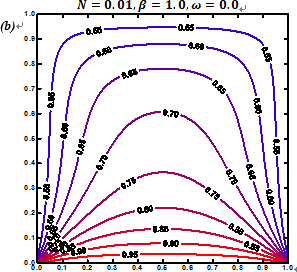
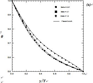
When radiation overcomes conduction [Figure 7(b)] (the case of $(N=0.01)$ the SS is attained fast and the temperature profile became nonlinear which is well observed in Figure 7(a). With increase in values of , we tend for a medium where the effects of radiation and conduction are the same $(N=1)$ [22]. The extinction coefficient which is the sum of the scattering albedo and the absorption coefficient represent the amount of attenuation by two different mechanisms:absorption and out-scattering. The higher the value of , the more optically participating the medium is. In Figure 8(a),non-dimensional distributions are plotted for the extinction coefficient $\beta=0.01,0.1$ and 1.0, respectively. For these results $\omega=0.0$ and $n=0.1$ , we can observe the effect of increasing in value of extinction coefficient in making the medium go for domination of radiation over conduction.
Figure 7. Steady state centerline temperature $\theta=T / T_{r e f}$ for different parameter (a) $\omega=0.0, \beta=1.0, \varepsilon_{S}=1.0$ and different values of conduction-radiation parameter $N,(b)-(d)$ thecorresponding isotherms
Figure 8. Steady state centerline temperature for different parameter (a) and different values of extinction coefficient , (b)-(d) the corresponding isotherms
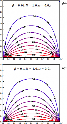
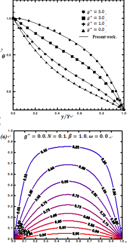
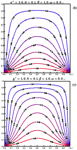
We investigate also the effect of heat generation [Figure 9(a)-(e)]. Heat generation will increase the non-linearity of temperature profile. Heat generation in the medium increases the effect of radiation. That’s why, when g+ increases,nonlinearity in the Steady-State profile will increase. For the results plotted in Figure 9(e), since heat generation is very intense near the hot boundary, dimensionless temperature is found to go beyond the unity value.
Figure $9 .$ (a) Steady state centerline temperature $\theta=T / T_{\text {ref}}$ for different parameter $\omega=0.0, N=0.1, \varepsilon_{S}=1.0$ and different values of heat generation rate $g^{+},(a)-(d)$ the corresponding isotherms
3.3 Variable thermal conductivity
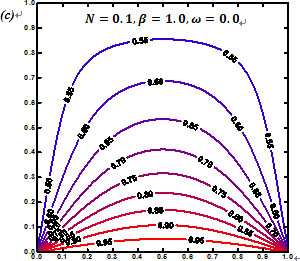
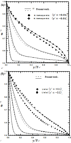
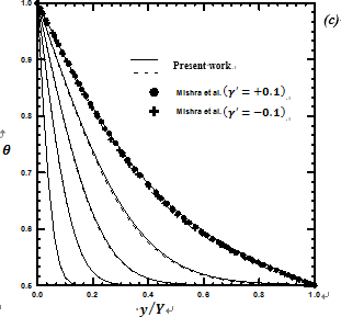
In this section, the variable Thermal conductivity case is adopted. In Figure 10(a)-(c), the effect of $\gamma=\gamma^{\prime} T_{r e f} N$ on temperature profile along the centerline $(x / L=0.5)$ are shown. The results are presented for different values of the conduction radiation parameter N and scattering albedo, . The results are in good agreement with those obtained by [23,24, 3]. From Figure 10(a)-(c), in radiation domination case,the effect of thermal conductivity on temperature profiles is found more pronounced. From the obtained results, one can conclude that the obtained results developing by a BGK LBM home code with the suggested conditions can produce reliable results. We furthermore extend the present formulation to deal with a convection heat transfer engineering problem with heat generation where the conductivity is variable.
Figure 10. Comparison of Centerline temperature =T/Tref
with those available in literature, (a) for N=0.01 and =0.5 with [23], (b) for N=0.1 and =0.0 with [24], (c) for N=1.0 and =0.0 with [3]
3.4. Natural convection with heat generation
We consider first the case of pure natural convection in a square enclosure in absence of heat generation and with constant thermal conductivity. The Chapman-Enskog method is adopted to provide the flow field under Boussinesq approximation. The geometry adopted is as in Figure 1(c).The walls at x=0.0 and x=L are kept at hot and cold temperature Th and Tc, respectively. The horizontals walls are under adiabatic boundary condition. With accordance to the grid analysis sensitivity done by [23], the mesh grid adopted in this simulation is (61 61).
Figure 12. Flow field at Pr=0.71 and Ra=1.89 105 (a) Isotherms, (b) Temperature profiles in comparison with [23]and [24]
In Figure 12(a)-(b), flow filed at Pr=0.71 and Ra=1.89 105 , namely isotherms and temperature profile are plotted. Good agreements with available results in literature are found. Then, the effect of heat generation and variation in thermal conductivity are taken into account. The flow assumption, are Pr=0.71 and Gr=20000. Where the Grashof number is defined as:
$G r=\frac{\rho^{2} g \beta \Delta T L^{3}}{\mu^{2}}$ (34)
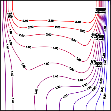
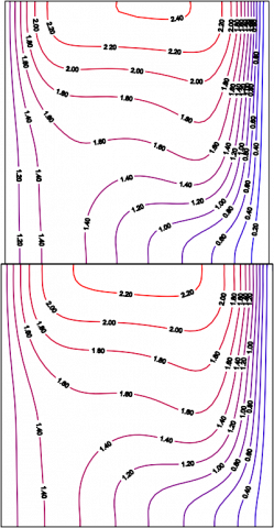
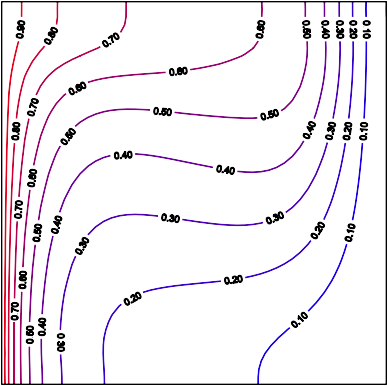
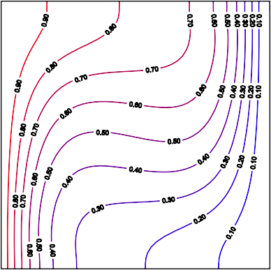
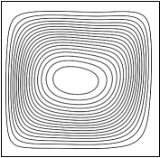
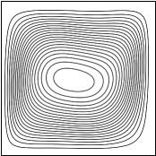
Figure 13. Isotherms for various flow conditions (a)
$g^{+}=25, \gamma=-0.25(b) g^{+}=25, \gamma=-0.1(c) g^{+}=25, \gamma=0.0$
$(d) g^{+}=0, \gamma=-1.5(e) g^{+}=0, \gamma=-1$ and $(f) g^{+}=0, \gamma=0$
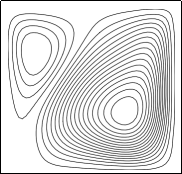
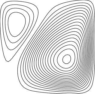
In Figure 13(a)-(f), isotherms for different values of $g^{+}$ and $\gamma$ are plotted. In Figure 12(a)-(c), isotherms are plotted for $g^{+}=25$ and various values of . The decrease in thermal conductivity coefficient induces an accentuation in nonlinearity of the thermal fluid flow. From Figure 13(b) it's clear that the temperature inside the enclosure is slightly increased than the boundary temperature due to the presence of internal heat generation. The corresponding streamlines for flow conditions of figure 13, are illustrated in Figure 14(a)-(f).When both $g^{+}$ and are taken into account, we can observe the presence of two vortices [Figure 14(a)-(c)]. With decrease of $g^{+}$, the smallest vortex near the cold wall, graduallydisappear.
Figure 14. Streamlines for various flow conditions
$g^{+}=25, \gamma=-0.25 \quad$ (b) $g^{+}=25, \gamma=-0.1$ (c) $g^{+}=25, \gamma=0.0$
(d) $g^{+}=0, \gamma=-1.5(e) g^{+}=0, \gamma=-1$ and $(f) g^{+}=0, \gamma=0$
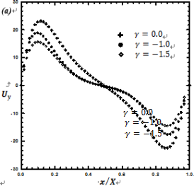
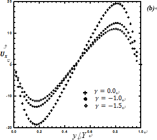
The effect of variation of thermal conductivity on mid-height x-velocity and y-velocity is depicted in Figure 15(a)-(b). With decrease in thermal conductivity, velocity decreases along the centerline axes
Figure 15. (a) Mid-height -velocity profiles and (b) Mid-height -velocity profiles for different values of variablethermal conductivity parameter $\gamma$
In this study, various heat transfer problems involving radiation and/or conduction and natural convection have been simulated with the lattice Boltzmann method. In addition to that, the case of variable thermal conductivity has been considered. Modified formulation of thermal lattice Boltzmann equation is used to emphasis the effect of variable thermal conductivity with temperature, on flow fields, under several conditions. This formulation is based on a modified equilibrium distribution function able to account for the variation of thermal conductivity with temperature.Comparisons were made against several reported data in literature and good agreements were found.
|
Cp |
specific heat capacity, ( J / KgK ) |
|
cs |
speed of sound, (m s) , |
|
D ei |
variable part of thermal diffusivity, (m2 s) lattice velocity vector in direction i |
|
fi (r ,t ) |
particle distribution function in the ith direction |
|
f eq (r ,t ) i |
equilibrium distribution function in the ith direction |
|
Gr |
Grashof number |
|
Ii ( xn ,t ) |
radiation intensity |
|
I eq ( x ,t ) i n |
equilibrium radiation intensity |
|
Pr |
Prandtl number |
|
N |
conduction-radiation parameter |
|
r |
position vector ( x, y), m |
|
Ra |
Rayleigh number |
|
t |
time, s |
|
wi |
weight factor in the ith direction |
|
wgi |
lattice constant in the direction ith for radiative equation |
|
x, y |
axial coordinates |
|
Greek symbols |
|
|
a0 |
constant part of the thermal diffusivity, (m2 s) |
|
b |
extinction coefficient |
|
g ' |
coefficient of thermal conductivity variation, 1 K |
|
t |
relaxation time, |
|
e w |
emissivity of the wall |
|
q |
non-dimensional temperature |
|
l |
thermal conductivity, W / mK |
|
l0 |
thermal conductivity at reference temperature Tref , W / mK |
|
r |
density, Kg / m3 |
|
Subscripts |
|
|
W , E, S, N |
west, east, south and north wall |
|
ref |
reference |
[1] Chu H.S., Tseng C.J. (1992). Conduction-radiation interaction in absorbing, emitting and scattering media with variable thermal conductivity, Journal of Thermophysics and Heat Transfer, Vol. 6, No. 3, pp.537-540. DOI: 10.2514/3.393
[2] Tseng C.J., Chu H.S. (1992). Transient combined conduction and radiation in an absorbing, emitting and anisotropic ally scattering medium with variable thermal conductivity, International Journal of Heat and Mass Transfer, Vol. 35, No. 7, pp. 1844-1847.
[3] Mishra S.C., Talukdar P., Trimis D., Durst F. (2005).Two-dimensional transient conduction and radiation heat transfer with variable thermal conductivity,International Communications in Heat and Mass Transfer, Vol. 32, Nos. 3-4, pp. 305-314. DOI:10.1080/10407780290059387
[4] Varmazyar M., Bazarga M. (2011). Modeling of free convection heat transfer to a supercritical flfluid in a square enclosure by the lattice Boltzmann method,ASME Journal of Heat Transfer, Vol. 133. DOI:10.1115/1.4002598
[5] Succi S. (2001). The lattice Boltzmann equation for flfluid dynamics and beyond, Clarendon Press, Oxford,pp. 3-16. DOI: 10.1016/S0997-7546(02)00005-5
[6] Yuang H.Z., Niu X.D., Shu S., Li M., Yamaguchi H.(2014). A momentum exchange-based immersed boundary-lattice Boltzmann method for simulating a flexible filament in an incompressible flow, Computers and Mathematics with Applications, Vol. 67, pp.1039-1056. DOI: 10.1016/j.camwa.2014.01.006
[7] Huang X.P., Chen Z.Q., Shi J. (2016). Simulation of solid-liquid phase transition process in aluminum foams using the Lattice Boltzmann method,International Journal of Heat and Technology, Vol.34, No. 4, pp. 694-700. DOI: 10.18280/ijht.340420
[8] Yao S.G., Lei L., Deng J.W., Lu S., Zhang W. (2015).Heat transfer mechanism in porous copper foam wick heat pipes using nanofluids, International Journal of Heat and Technology, Vol. 33, No. 3, pp. 133-138.DOI: 10.18280/ijht.330320
[9] Talukdar P., Mishra S.C. (2010). Transient conduction and radiation heat transfer with variable thermal conductivity, Numerical Heat Transfer, Part A: Applications: An International Journal of Computation and Methodology, Vol. 41, No. 8, pp.851-867. DOI: 10.1080/10407780290059387
[10] Mishra S.C., Krishna N.A., Gupta N., Chaitanya G.R.(2008). Combined conduction and radiation heat transfer with variable thermal conductivity and variable refractive index, International Journal of Heat and Mass Transfer, Vol. 51, pp. 83-90. DOI:10.1016/j.ijheatmasstransfer.2007.04.018
[11] Hazi G., Markus A. (2008). Modeling heat transfer in supercritical fluid using the lattice Boltzmann method,Physical Review E, Vol. 77, pp. 1-10. DOI:10.1103/PhysRevE.77.026305
[12] Ginzburg I. (2006). Variably saturated flow described with the anisotropic lattice Boltzmann methods,Comput. Fluids, Vol. 35, No. 8-9, pp. 831-848. DOI:10.1016/j.compfluid.2005.11.001
[13] Mishra S.C., Talukdar P., Trimis D., Durst F. (2003).Computational efficiency improvements of the radiative transfer problems with or without conduction,a comparison of the collapsed dimension method and the discrete transfer method, Int. J. Heat Mass Transfer, Vol. 46, pp. 3083-3095. DOI:10.1016/S0017-9310(03)00075-9
[14] Chaabane R., Askri F., Ben N.S. (2011). Analysis of two-dimensional transient conduction-radiation problems in an anisotropic ally scattering participating enclosure using the lattice Boltzmann method and the control volume finite element method, Journal of Computer Physics Communications, Vol. 182, pp.1402-1413. DOI: 10.1016/j.cpc.2011.03.006
[15] Chaabane R., Askri F., Ben N.S. (2011). Parametric study of simultaneous transient conduction and radiation in a two-dimensional participating medium,Communications in Nonlinear Science and Numerical Simulation, Vol. 16, pp. 4006-4020. DOI:10.1016/j.cnsns.2011.02.027
[16] Chaabane R., Askri F., Ben N.S. (2011). Application of the lattice Boltzmann method to transient conduction and radiation heat transfer in cylindrical media, Journal of Quantitative Spectroscopy and Radiative Transfer, Vol. 112, pp. 2013-2027. DOI:10.1016/j.jqsrt.2011.04.002
[17] Asinari P., Mishra S.C., Borchiellini R. (2010). Alattice Boltzmann formulation to the analysis of radiative heat transfer problems in a participating medium, Numerical Heat Transfer, Part B, Vol. 57, pp.126-146. DOI: 10.1080/10407791003613769
[18] Di Rienzo A.F. (2012). Mesoscopic numerical methods for reactive flows: lattice Boltzmann method and beyond, PhD dissertation, Politecnico Di Torino,Italy.
[19] Mishra S.C., Kim M.Y., Maruyama S. (2012).Performance evaluation of four Radiative transfer methods in solving multi-dimensional radiation and/or conduction heat transfer problems, International Journal of Heat and Mass Transfer, Vol. 55, pp. 5819-5835. DOI: 10.1016/j.ijheatmasstransfer.2012.05.078
[20] Wu C.Y., Ou N.R. (1994). Transient two-dimensional radiative and conductive heat transfer in scattering medium, International Journal of Heat and Mass Transfer, Vol. 37, pp. 2675-2686.
[21] Yuen W.W., Takara E.E. (1988). Analysis of combined conductive-radiative heat transfer in a twodimensional rectangular enclosure with a gray medium,Journal of Heat Transfer, Vol. 110, pp. 468-474. DOI:10.1115/1.3250509
[22] Maroufi A., Aghanajafi C. (2013). Analysis of conduction radiation heat transfer during phase change process of semi-transparent materials using lattice Boltzmann method, Journal of Quantitative Spectroscopy and Radiative Transfer, Vol. 116, pp.145-155. DOI: 10.1016/j.jqsrt.2012.10.019
[23] Varmazyar M., Bazargan M. (2013). Development of a thermal lattice Boltzmann method to simulate heat transfer problems with variable thermal conductivity,International Journal of Heat and Mass Transfer, Vol.59, pp. 363-371. DOI:10.1016/j.ijheatmasstransfer.2012.12.014
[24] Li G.J., Ma J., Li B.W. (2015). Collocation spectral method for the transient conduction-radiation heat transfer with variable thermal conductivity in twodimensional rectangular enclosure, Journal of Heat Transfer, Vol. 137. DOI: 10.1115/1.4029237
[25] Barakos G., Mitsoulis E., Assimacopoulos D. (1994).Natural convection flow in a square cavity revisited:laminar and turbulent model with wall functions,International Journal for Numerical Methods in Fluids, Vol. 18, pp. 697-719. DOI:10.1002/fld.1650180705