OPEN ACCESS
In spite of evident differences, Constructal Theory and Thermoeconomics (in particular thermoeconomic optimization) have also some similarities. For instance, they both suggest the optimal allocation of two different types of losses: high permeability vs. low permeability flow losses in the Constructal Theory, while local losses inside the process vs. external losses for making available all resources actually consumed, at local level, by a component or a process in the thermoeconomic optimization. The paper discusses this one and related aspects, highlighting how the optimal criterion of minimum energy cost of the product can be derived from the Constructal Law, when the flow of useful product through the productive structure is considered as the characteristic flow of the system. In this context, the evolution of energy systems toward highly interrelated productive structures, with recycling flows, can be regarded as a consequence of the Constructal Law.
Thermoeconomics, Constructal Law, Exergy cost, Recycling.
In principle, Second Law (exergy) analysis can be applied to any kind of energy system, which is synthetically described in this approach as a network of energy flows, connecting some nodes (named components, or sub-systems) where different kinds of irreversible energy conversion processes may occur. This point of view is widely adopted for analyzing both natural, biological and ecological systems, and human-made, technological production systems [1-4].
Thermoeconomics may be regarded as a further step after exergy analysis, where external exergy destruction is taken into account for owning, maintaining and operating the components that make up a generic energy system, by means of some kind of cost [5-9]. In this approach, the exergy flows are not regarded as physical streams that flow in a real space (as is usual in the Constructal Theory approach), but rather as the functional relations among components, in the abstract space of possible productive interconnections, that make up the so called Productive Structure of the energy system.
In spite of these differences, Constructal Theory and Thermoeconomics (in particular thermoeconomic optimization) have also some similarities. For instance, they both pursue the optimal allocation of two different type of losses: high permeability vs. low permeability flow losses in the Constructal Theory, while local losses inside the process vs. external losses for making available all resources actually consumed, at local level, by a component or a process in the thermoeconomic optimization. These local resources include at least the energy and material flows required by the production, as well as the capital expenditure for owning, maintaining and operating the components that make up the system.
As it is evident in Literature, the Constructal Low can be used to predict the shape and structure for a lot of physical flow systems; the aim of the paper is to apply it to the productive structure of an energy system, in order to understand what can be inferred about the evolution of the functional relations among components.
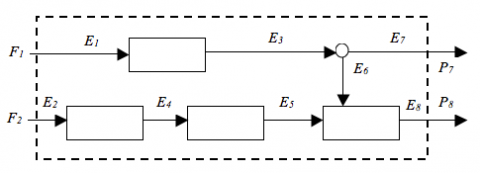
Let’s consider a steady state operation of a generic multi-component energy system and let's assume first that energy flows only are enough for completely describe its behavior (Fig. 1). If the energy flows inside the network are defined in order to properly describe the productive relations among components and with the outside of the system, each component (or process) can be regarded, at local level, as an autonomous production unit, having one output flow named Product or Function and one or more input flows, named Fuels or internal resources (multi-product components can be also considered, but with some restrictions about the formulation of the mathematical model of these kind of components [7]). As a result, a sort of local model of each component is isolated from the thermodynamic model of the whole system, while the network obtained can be regarded as the so called Productive Structure (PS) of the system. Each flow Ei describing a productive relation among components has to be defined on the basis of heat, work and mass flow rates and of thermodynamic conditions of working fluids inside the system. From a mathematical point of view, the choice of its analytic formulation is free, but exergy based productive relations have to be regarded as the general option [5].
Let’s consider the basic question: How much primary energy (or better, exergy) has been used by the macro-system to maintain each flows of the PS at a defined value? If the system is similar to a linear chain (like the one in Fig.1) and it is operating in stationary condition, the answer can be easily inferred [10]. In fact, flows E1 and E2 do correspond to the
primary energy F1 and F2, respectively; flow E3is maintained by F1, so that its unit energy cost is defined as k*3 = F1/ E3, and a similar situations happens for flows E4 and E5, too.
Let’s think at the bifurcation of flow E3 as a split, without any thermodynamic transformation or process, therefore the flow E7 results maintained by a fraction E7/ E3 of flow F1 and its unit cost is defined as k*7 = (E7/ E3) (F1/ E7) = k*3. Flow E8 is maintained by the remaining part of flow F1 and by the entire flow F2. Its unit cost is k*8 = k*3 (E6/ E8) + k*5 (E5/ E8).
Figure 1. A simple linear system with a split
The ratios like F1/ E3 º k31 (or E6/E8 º k86) can be defined as the specific exergy consumptions (or the partial specific consumptions) for obtaining a certain exergy flow inside the system. This approach is formalized in deep detail in [8], where a very elegant matrix formulation is introduced. In matrix form, the input/output relations for all components or processes inside the PS, as well as all unit exergy costs, can be expressed as follows:
$\boldsymbol{E}=^{t} \boldsymbol{K} \boldsymbol{E}+\boldsymbol{\omega}$(1)
$\boldsymbol{k}^{*}=\left[\boldsymbol{U}_{D}-\boldsymbol{K}\right]^{-1} \cdot \boldsymbol{k}_{e}^{*}$(2)
where K is a square matrix containing the specific exergy consumptions kij, while w and are vectors containing the out coming products (required by external users) and the unit exergy costs of the incoming energy resources, respectively. Notice that the latter have to be equal to one if the incoming resources are actually primary energy resources, like solar radiation. Eq. (1) is named the Characteristic Equation of the PS.
In principle, the approach could be the same also if some incoming resources were not energy or material resources (measured by their exergy content), but capital expenditure for owning, maintaining and operating the components that make up the system. These kind of production factors are generally not known in term of their exergy content, or exergy cost, but they can be easily converted in monetary flows [€/s], so that the classical thermoeconomic approach prescribes to transform all costs in monetary flows by means of the unit monetary costs of all energy and material inputs.
In alternative, accounting methods based solely on exergy have been proposed by various Authors, beginning by Szargut [11, 12] and today the option of defining an exergy equivalent of money is widely accepted and adopted in literature [13, 14]. The idea that an exergy equivalent of money can be defined and used in exergy cost accounting will be taken into account in the following, without further considerations (an interesting discussion about accounting methods based solely on exergy and the proper definition of the exergy equivalent of money, for a generic economy, is reported in [15]).
Let’s consider the component producing the flow E3 in Fig. 1 and consuming the flow E1, which is regarded as a primary energy resource (F1). It is trivial to notice that its product flow per unit of resource consumption is equal to the inverse of the unit exergy cost of its product:
$\frac{E_{3}}{F_{1}}=\frac{1}{k_{3}^{*}}$(3)
This result can be easily demonstrated for all flows in whatever productive structure, provided that the unit exergy costs (k*i) are obtained from eq. (2); it can be also inferred that:
$\frac{P_{j}}{I_{T O T_{j}}}=\frac{1}{k_{j}^{*}-1}$(4)
where ITOTj is the total exergy destruction caused by the production of the flow Pj, inside and outside the component actually producing that product (Pj); the external exergy destruction IEXTj is the summation of all irreversibility produced for making available the local resources Ei, required by the component in hand, tracked back to the primary energy resources:
$I_{E X T_{j}}=\sum_{i}\left(k_{j}^{*}-1\right) E_{i}$(5)
In addition, it can be also inferred that the external exergy destruction for producing Pj is greater than the internal one if the unit exergy cost k*j and the specific exergy consumptions kij of the component producing Pj fulfill the following relation:
$k_{j}^{*} \geq 2 \sum_{i}\left(\kappa_{i j}-1\right)$(6)
As it is well known, the Constructal Law, proposed by Bejan in 1996, states [16]:
For a finite-size flow system to persist in time (to live), its configuration must evolve in such a way that provides greater and greater access to the currents that flow through it.
If the current that flow through the energy system is identified with its useful product (per unit of primary exergy resources consumed) the Constructal Law prescribes an evolution toward a product increase, i.e. (in thermoeconomic terms) an evolution toward a reduction of the unit exergy cost of the product (Eq. 3). This is exactly the aim of the thermoeconomic analysis. In other words, the axiom of thermoeconomic analysis: reduce the unit exergy cost of the products, can be inferred from the Constructal Law if the energy system is described in thermoeconomic terms and the current that flow through it is identified with the flow of its useful product.
Let’s consider now a generic real energy system: it is straightforward to think that it does not operate in an empty space (like the system in Fig. 1) but that it is surrounded by a biosphere (or an anthroposphere) where different kinds of resources are available at different unit exergy costs and with different constraints about their availability in time and space. This way of thinking may be named as the system in its thermoeconomic environment. In order of reducing the unit exergy cost of its product, the system may evolve to reduce its specific exergy consumptions of local resources (kij), or it can modify its supply chain, using resources with a lower unit exergy cost. Neither of these strategies should be preferred over the other, because the internal irreversibility can be either greater or smaller than the external ones, as can be inferred from Eq. 6.
To illustrate the evolution of a possible energy system in its thermoeconomic environment, the framework shown in Fig.2 is considered. In particular, a solar system, made up of three sub-systems, is highlighted inside the dashed rectangle. Natural resources (E2) are used, after extraction and transportation (E6), for manufacturing a solar energy conversion system (let’s think, for instance, a photovoltaic or a concentrated thermodynamic solar system); than it is used for converting the solar radiation (E1) into electric power (E8).
The thermoeconomic environment includes three big sub-systems only: the fuel industry, supplying fossil fuel (E5) for extraction and transportation of row mineral resources, for the industrial plant production (E9) and for the power plants operation (E10); a set of power plants, supplying electric energy to all power users (E7and E11-E14) and the industrial plant production, supplying all fixed capital required by the other productive phases (Z1-Z4), except by the direct solar energy conversion (Z5), whose fixed capital is produced inside the control volume of the solar system.
Notice that, in this illustrative example, the exergy equivalent of money can be calculated from the cost balance of the industrial plant production, given that fixed capital is taken into account by means of monetary flows [€/s], calculated on the same time basis of the exergy flows.
Figure 2. A solar energy system in a possible thermoeconomic environment
A lot of other sub-systems and productive relations could be added, in order of defining a more meaningful thermoeconomic environment, but they are outside of the objectives of the illustrative example. For the same reason, the actual values of the flows in Fig. 2 are not of interest.
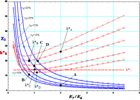
Figure 3. Relation used for evaluating the fixed capital Z2 and the corresponding values of the unit exergy cost k*8
To show some kind of evolution, consistent with the Construcal Law, let’s assume in the following that the thermoeconomic environment outside the solar system does not vary, whilst the solar system can modify the fixed capital (Z2) and the electric power (E7) required by the manufacturing of the energy conversion components. As is usual in the ambit of thermoeconomics (see, for instance, [17]) a trade-off is introduced between the capital intensity (Z2/E6) and the energy intensity (E7/E6) of the production process, at constant quality of the product, i.e. without modifying the energy conversion efficiency (E8/E1) of the solar system that is produced in the component manufacturing phase and then is operating in the energy conversion phase. A possible technological development (or improved energy conversion strategy) is also taken into account, by introducing the hypothesis that a similar trade-off exists also at energy conversion efficiencies higher than the reference one (equal to 12%), but it implies also a higher consumption of local resources (capital and/or exergy). Therefore, the following relation is used for evaluating the fixed capital Z2:
$\frac{Z_{2}}{E_{6}}=\frac{1}{\left(\frac{E_{7}}{E_{6}}\right)^{n}} \frac{m}{\left(\frac{E_{1}}{E_{8}}\right)-\frac{1}{\eta_{M}}}$(7)
where n and m are proper constants and hM is the maximum possible efficiency considered. In Fig. 3, Eq. 7 is reported in form of curves Z2 = f (E7/E6), by using the efficiencyh8 = E8/E1 as a parameter. In the same Figure, the corresponding values of the unit exergy cost k*8 are also shown by using the same parameter, jointly with the constant value of k*7 as a reference.
Let’s consider a starting workable condition (A), where the solar system is based on an energy conversion phase with an efficiency h8 = 12%. As can be seen in Fig.3, the electric power E8 is produced at a unit exergy cost k*8 greater than the unit exergy cost k*7 of the power consumed in the component manufacturing phase. This is clearly not profitable from a thermoeconomic point of view, but it may correspond as well to a real situation, because of some constraint about the availability in time or space of energy resources produced with higher efficiency, or because of some regulatory prescription of the energy market.
As shown in the previous paragraph, the Constructal Law prescribes an evolution of the system toward a condition allowing lower unit exergy costs to be obtained. This can be achieved approaching condition (B), which is the minimum of the curve at constant parameter h8 = 12%, therefore it can be identified as the optimal trade-off between the capital intensity and the energy intensity of the production process, without modifying the energy conversion efficiency h8. This kind of evolution corresponds to the thermoeconomic optimization of the system, in order of obtaining a greater and greater flow of useful product, per unit of primary exergy resources consumed.
In the Constructal Law language, it would be said that the optimal allocation of two different types of losses has been obtained in the optimal thermoeconomic condition (B): local losses inside the control volume of the system vs. external losses in the thermoeconomic environment, for making available all resources actually consumed by the system itself. Therefore, this result can be regarded as analogous to the optimal allocation of losses between high permeability and low permeability flows in a river basin, or in a lot of other tree shaped structure, obtained in Literature on the basis of the Constructal Law (see, for instance [16] and the references reported there).
In the example in hand, the optimal thermoeconomic condition (B) requires a lower energy intensity and a higher capital cost, but this is related with the starting workable condition (A) on the right hand side of point (B).
Going on towards lower and lower unit exergy costs of the power produced, implies a technological development (or an improved energy conversion strategy) allowing the system to achieve a higher energy conversion efficiency h8.
In the example shown in Fig. 3, an energy conversion efficiency h8 = 20% allows a further reduction of the unit exergy cost k*8 in a wide range of energy intensities (E7/E6), with a minimum corresponding to condition (C).
Notice that in condition (C) in Fig. 3, the unit exergy cost k*8 has reached a value as low as the reference value k*7 of the power consumed in the component manufacturing phase. This is a crucial condition, because it means that now there are two option for obtaining the electric power required by the component manufacturing phase, at the unit exergy cost k*7 (=k*8): using the product of the power plant considered
along with the evolution from condition (A) to condition (C), or split the product E8 of the solar energy system itself in two flows, the first one for the power users and recycling back the second one, in order of replacing the previous external flow E7. In this second option, a recycling flow arises in the productive structure, in consequence of the evolution prescribed by the Constructal Law.
It can be easily shown that a further improvement of the energy conversion efficiency (for instance, h8 = 25%) allows a further reduction of the unit exergy cost k*8, in a wide range of energy intensities (E7/E6), even if the recycling flow do not occur (in this case, condition (D) can be reached); but it is evident that a better result can be obtained with the partial recycling of flow E8, because it is a resource made available with a lower total exergy destruction (Fig. 4).
Figure 4. The unit exergy cost k*8, with and without the partial recycling of flow E8
This is an important point, because it means that, once the recycling flow has arisen, the selection criteria expressed by the Constructal Law works in the direction of reinforcing the recycling flow itself.
Notice that such conclusions can be inferred in force of the framework of the system in its thermoeconomic environment, where different kinds of resources are available at different unit exergy costs and with different constraints about their availability in time and space. In this framework the system is free, subject to the mentioned constraints, of switching to use local resources at a lower unit exergy cost, so as to increase its flows of useful product (per unit of primary exergy resource consumed), as prescribed by the Constructal Law. If the energy system is supposed to operate inside an empty space, there are no choice about the local resources to be employed, and the Constructal Law does not find any degree of freedom to morph the productive structure and to make the recycling arise.
In the previous paragraph, the hypothesis has been introduced stating that the production of solar energy conversion systems with higher efficiencies implies an higher consumption of local resources (capital and/or exergy). Finally, notice that, if this hypothesis were replaced with a different one implying constant, or even lower, consumption of local resources, the recycle would arise even more easily.
Taking into account that in a real energy system the chance for introducing recycling flows are much more, the expectation is that these results could be extended to all generic energy systems (both technological and biological) stating:
The Constructal Law prescribes the evolution of energy systems toward highly interrelated productive structures, with multiple recycling flows, at different hierarchical level.
The Constructal Law can be used to predict the shape and structure of a lot of physical flow systems; in this paper it has been applied it to the productive structure of an energy system, in spite of being the latter a network of functional relations among components (in the abstract space of possible productive interconnections), rather than a stream of physical flows.
If the energy system is described thought its productive structure, as in the thermoeconomic approach, and the current that flows through it is identified with its useful product (per unit of primary exergy resources consumed), the Constructal Law prescribes an evolution toward a reduction of the unit exergy cost of the product, that is strictly consistent with the aim of the thermoeconomic analysis.
This can be achieved approaching the optimal allocation of two different types of losses: local losses inside the control volume of the system vs. external losses in the thermoeconomic environment, for making available all resources actually consumed by the system itself. In the thermoeconomic language, this is the optimal trade-off between the capital investment and the exergy destruction of the production process, and corresponds to the thermoeconomic optimization of the system.
In consequence of the evolution prescribed by the Constructal Law, it has been highlighted that recycling flows may arise in the productive structure and, once a recycling flow has arisen, the selection criteria expressed by the Constructal Law works in the direction of reinforcing the recycling flow itself. In this process, a crucial role is played by the framework of the thermoeconomic environment, because, if there are no choices about the local resources to be employed, the Constructal Law does not find any degree of freedom to morph the productive structure and to make the recycling arise.
In the outlined context, the evolution of energy systems toward highly interrelated productive structures, with multiple recycling flows, can be regarded as a consequence of the Constructal Law.
1. A. Bejan, G. Tsatsaronis and M. Moran, Thermal Design and Optimization (New York: John Wiley & Sons, 1996).
2. Odum T.H., Emergy Accounting, 2000, Centre for Environmental Policy Environmental Engineering Science University of Florida, Gainesville. DOI: 10.1007/0-306-48221-5_13.
3. Ulgiati, S. and Brown, M.T., “Emergy accounting of human-dominated, large-scale ecosystems,” Thermo-dynamics and Ecological Modelling, Jorgensen Ed., 2001, Lewis Publisher, London.
4. Brown M.T. and Herendeen R.A., “Embodied energy analysis and EMERGY analysis: a comparative view,” Ecological Economics, Vol. 19, 1996, pp. 219-235. DOI: 10.1016/S0921-8009(96)00046-8.
5. Gaggioli R.A., “Second law analysis for process and energy engineering,” Efficiency and Costing, ACS Symposium Series Vol. 235, 1983, pp. 3–50.
6. El-Sayed Y.M., Gaggioli R.A., “A critical review of second law costing methods: Parts I and II,” ASME Journal of Energy Research Technology, Vol. 111, 1989, pp. 1–15.
7. Reini M., Lazzaretto A., Macor A., “Average structural and marginal costs as result of a unified formulation of the thermoeconomic problem,” Proc. of Int. Conf. Second Law Analysis of Energy System Towards the 21st Century, E. Sciubba, M.J. Moran Eds, Esagrafica Roma, 1995.
8. Valero A., Lozano M.A., Munoz M., “A general theory of exergy savings, Part I: On the exergetic cost, Part II: On the thermoeconomic cost, Part III: Energy savings and thermoeconomics,” Computer-Aided Engineering of Energy Systems, Vol. 2–3. New York: ASME; 1986, pp. 1–21.
9. Tsatsaronis G., Winhold M., “Exergoeconomic analysis and evaluation of energy conversion plants,” Energy, Vol. 10, 1985, pp. 69–80.
10. Gaggioli R. and Reini M., “Connecting 2nd law analysis with economics, ecology and energy policy,” Entropy, 2014, 16(7), 3903-3938. DOI: 10.3390/e16073903.
11. Szargut J., Morris D.R., Steward F.R., Exergy Analysis of Thermal, Chemical, and Metallurgical Processes, Hemisphere, 1988.
12. Szargut J., Exergy Method: Technical and Ecological Applications, WIT Press; 2005.
13. Sciubba E., “Beyond thermoeconomics? The concept of Extended Exergy Accounting and its application to the analysis and design of thermal systems,” Exergy, The International Journal, Vol. 1 (No. 2), 2001, pp 68-84. DOI: 10.1016/S1164-0235(01)00012-7.
14. Sciubba E., “Engineering Economics to Extended Exergy Accounting: A possible path from monetary to resource-based costing,” J. Ind. Ecology, Vol. 8, No. 4, 2004. DOI: 10.1162/1088198043630397.
15. Rocco M.V., Colombo E., Sciubba E., “Advances in exergy analysis: a novel assessment of the Extended Exergy Accounting method,” Applied Energy, Vol. 113, January 2014, pp 1405-1420. DOI: 10.1016/j.apenergy.2013.08.080.
16. Bejan A. and Lorente S., “Constructal law of design and evolution: Physics, biology, technology, and society,” J. Appl. Phys., 113, 151301, 2013. DOI: 10.1063/1.4798429.
17. Tsatsaronis, G., Exergoeconomics and Exergo-environmental Analysis, Bakshi, B.R., Gutowski, T.G., Sekulic, D.P. (Eds.) Thermodynamics and the Destruction of Resources, Cambridge University Press, New York, 2011, Chapter 15, pp. 377–401. DOI: 10.1017/CBO9780511976049.