OPEN ACCESS
Open flow network is a weighted directed graph with source and sink to depict flux distributions in the steady state of an open flow system. Energetic food webs, global trade networks, input-output networks and clickstreams, are open flow network models of energy flows, goods flows, money flows, and collective attention flows respectively. Based on the Markov chain techniques, a set of quantities, such as influx, total through-flow, dissipation flow, first-passage flow distances, and first-passage flows can be defined to characterize flows and interactions between nodes. Under this framework, some universal patterns have been found in open flow networks, such as allometric scaling law, generalized Kleiber law, dissipation law, and gravity law, etc. We suppose constructal law cannot only be applied to flow systems with explicit spatial structures like rivers, vascular networks, animal movements, but also can be applied to open flow networks without explicit spatial structures such as energetic food webs, input-output networks, and clickstreams of attention flows. We try to formulate constructal law in the open flow network framework and test it by the real data.
Open flow network, Allometric law, Dissipation, Constructal law.
Complex networks surround us — from national power grids and airline networks to social contact disease networks, neuronal networks and protein-protein interactions [1-4]. However, due to the limitation of the traditional binary graphs for describing the complexity of the various real systems, more networks, as weighted networks [5-6], bi-partite graphs [7], temporal networks [8] for instance, are emerging in the past decade as novel extensions of graphs. Especially, open flow network as a particular kind of directed weighted networks to depict the open flow system plays an important role in flow systems.
As we all known, openness and flowability are the most significant features in the open complex systems in common. On one hand, The system needs to exchange energy and material with environment [9] to maintain itself in the ordered state. On the other hand, Energy and material flows are delivered to each unit of a system by the flow network [10-11]. Open flow network is an ideal tool to understand open flow systems, in order to answer the questions like system stability, transportation efficiency in a quantitative way. The distribution of these flows in the entire body of a system is described by directed weighted edges. Two special nodes which called ”source” and “sink” are added to represent the external environment of the system and to reflect the openness of the system. Because the flow system is supposed to be in a steady state, the flow network is always balanced which means that the total inflow of each node equals to its total out flows except for the source and the sink. We also abbreviate open flow network as flow network in this paper.
Economic input-output model [12] proposed by the famous economist Leonief [13-14] in 1950s is essentially an open flow network indeed. Input-output relation-ship between industries can be seen as a kind of flows(money or material), and all of them are conservative. Money flows from the final demands compartment, circulates in different sectors of an economic system, and eventually flows to the value added compartment(or goods flow in an inverse direction) [15]. Thus, value-added compartment can be regarded as the sink, and final demands sector can be regarded as the source.
Energetic food web is another typical example of the flow network. H. T. Odum [16-17] used to engage in depicting energy flows between species due to the predatory interactions in an ecosystem as a circuit. The sunlight is the source of energy for the whole system, and all the energy will be converted to the waste heat by respiration and dissipation. Later on, Patten et. al put forward a systematic “Ecological Flow Analysis” method [18-22] to investigate energetic food webs in ecosystem. They not only proposed a series of methods to measure the direct or indirect interactions, but also gave a bunch of indices to depict the flow properties of circulation of the food webs [23-26].
Other examples of open flow networks include trade networks, clickstream networks [27,28] and so on. In the trade networks [29], each node represents the country in transactions and the flux means the volume of a trade between two countries. While in the clickstream networks, the node denotes a web, and the flux is the times of the successive clicks between two webs. Anyhow, open flow networks can provide a unified view to understand a variety of open flow systems.
2.1 Mathematical representation
In this section, we will give a mathematical description of open flow network. As mentioned above, an open flow network is a special directed weighted network, in which weight denotes flow. Fig. 1 is a simple example:
Figure 1. A simple example of flow network. The number beyond the edges is the flow, and the orientation of the edges is the flow direction
Any open flow network can be represented as a flow matrix F={fij}, here, fij means the flow from i to j. The two special node source and sink, respectively denoted by 0 and N+1( where N is the total amount of the nodes in the network except for source and sink). In flow matrix, we stipulate that the first row and the first column correspond to the source, and the last row and column correspond to the sink. Because the source has no inflow , all the elements in the first column are all 0s. Similarly, all the elements in the last row corresponding to the sink are also 0s. Therefore the flow matrix of the network in Fig. 2 can be shown as below.
|
|
Source |
1 |
2 |
3 |
4 |
5 |
sink |
|
|
0 |
80 |
0 |
0 |
0 |
0 |
|
|
1 |
0 |
0 |
50 |
30 |
0 |
0 |
0 |
|
2 |
0 |
0 |
0 |
0 |
20 |
30 |
10 |
|
3 |
0 |
0 |
10 |
0 |
0 |
0 |
25 |
|
4 |
0 |
0 |
0 |
0 |
0 |
10 |
10 |
|
5 |
0 |
0 |
0 |
5 |
0 |
0 |
35 |
|
sink |
0 |
0 |
0 |
0 |
0 |
0 |
0 |
|
|
|
|
|
|
|
|
|
Figure 2. The flow matrix of the Fig. 1
2.2 Flow balance condition
Open flow networks are always balanced because they are used to represent the system in a steady state. Therefore, for any node except the source and the sink, the summation of inflows equals to the summation of its outflows and we call this balance condition. We can describe it with the formula:
$\sum_{j=0}^{N} f_{j i}=\sum_{j=0}^{N+1} f_{i j}, \quad 1 \leq i \leq N$(1)
Because the flow network is balanced, we can then define an N * N matrix M from F follows:
$m_{i j}=\frac{f_{i j}}{\sum_{k=1}^{N+1} f_{i k}} \quad, \quad \forall i, j \in[1, N]$(2)
Where, mij represents the transition probability that a flowing particle transfers from i to j after it visiting i. Thus, the flow network can be also treated as a Markov chain, and the matrix M is called the Markov matrix.
Another important matrix which will be used widely is called the Fundamental matrix, it can be expressed by the Markov matrix as
$U=I+M+M^{2}+\cdots=\sum_{i=0}^{\infty} M^{i}=(I-M)^{-1}$(3)
Where I is the unity matrix. Any element uij in U matrix denotes the influence from i to j along all possible pathways including direct and indirect paths.
Thus, several important quantities defined on the open flow networks can be expressed by M and U.
2.3 Basic quantities
In this subsection, we will introduce several basic quantities on flow networks.
2.3.1 Total Throughflow Total throughflow is the total flux through any node. Because the network is balanced, node i’s total throughflow Ti is identical to the gross inflow $\sum_{j=0}^{N} f_{j i}$, and the gross outflow $\sum_{j=0}^{N} f_{j i}^{\sum_{j=0}^{N} f_{j i}}$. that is :
$T_{i}=\sum_{j=0}^{N} f_{j i}=\sum_{j=1}^{N=1} f_{i j}$(4)
2.3.2 Dissipation The dissipation of node i is defined as the flow from i to the sink, that is:
$D_{i}=f_{i, N+1}$(5)
In most open flow networks, dissipations always have very large proportions to the total throughflows [22].
2.3.3 Node’s Impact Ci is also an vertex-related index, it reflects the total indirect effects. If all the particles that flow through node i will be dyed red, then Ci is just the number of the red particles in the network. It seems that the larger the Ci is, the greater node i’s influence to the entire network. Therefore, Ci is interpreted as the impact of node i [30]. it can be calculated as:
$C_{i}=\sum_{k=1}^{N} \sum_{j=1}^{N}\left(f_{0 j} u_{j i} / u_{i i}\right) u_{i k}$(6)
f and u are the elements of flow matrix and fundamental matrix U. The variable Ci is extended from the approach of Garlaschelli et al. [31] to calculate the allometric scaling of food webs.
3.1 Allometric law
Allometric law is a universal law in flow systems. It describes a set of power law relationships between various features of organisms such as metabolism, heart rate, etc. and their body mass. Particularly, the biologist Kleiber has found that an organism’s metabolism F, and its size M follow a three quarters power law which is also named Kleiber’s law [32].
Banavar et al. and Garlaschelli et al. further pointed out that Kleiber law can be explained by a self-similar tree embedding the organism’s body [11,31]. And the self-similarity of this tree can be characterized by an allometric scaling for nodes.
Although the structures of open flow networks are much more complicated than trees, the similar allometric law can also be found. However, there two types of allometries in flow networks, namely the allometric scaling for one single flow network, and the allometric growth for the growth of network.
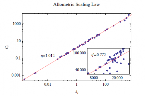
3.1.1 Allometric scaling The allometric scaling of a flow network is a power relationship between Ci and Ti, it can be written as:
$C_{i} \propto T_{i}^{\eta}$(7)
η is the exponent of the allometric scaling. This scaling reflects the self-similar nature of flow networks, and the exponent indicates the hierarchicality of the flow network. We found that this pattern is ubiquitous for almost all the flow networks that we have collected, and their exponents are very different for different types of networks.
Fig.3 shows the scaling between Ci and Ti for Mondego energetic food web. In the figure, Ti represents the metabolism of node i, and Ci is the equivalent body mass of the sub-system rooted from vertex i.
Figure 3. Allometric scaling law for the ecological network and the null model (inset)
To test whether the allometric scaling pattern is significant compared to random flow networks, we build a null model in which the numbers of nodes and edges are maintained, all links are re-connected randomly and all flows on edges are also randomly assigned on the interval (0,fm) evenly, where fm is the maximum flux of the original network. From the inset of Fig. 3. we can note that the null model network does not show a significant allometric scaling law.
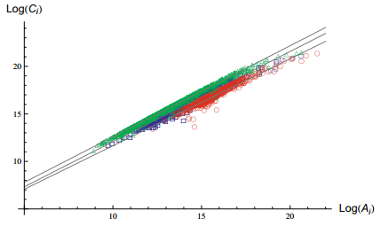
The same allometric scaling law can be found in clickstream networks as shown in Fig. 4,
Figure 4. The allometric scaling in the three clickstream networks of the top 1000 websites for different periods. The data points from three networks are plotted in different colours and styles. The values of η are 0.95, 0.92 and 0.96, respectively
We found the allometric scaling is also ubiquitous across the three studied flow networks. Nodes in different colours correspond to different networks. The values of η are estimated to be in the range of 0.92~0.96 and all of them are smaller than 1,which are distinct from that in the ecological flow networks.
As demonstrated above, the exponent η reflects the degree of centralization of the whole flow network, and also depicts the shape of an open flow network: hierarchical or flat. We can roughly classify the flow networks that we have studied into three universal classes according to the exponent, as shown in table 1:
Table 1. The comparison of different open flow networks with exponent η
|
network |
η |
classes |
implication |
|
Ecosystem network |
≈1 |
neutral |
The impact of species is proportional to their flows |
|
Clickstream network |
<1 |
flat |
The impact of large websites do not match with their flows |
|
Industrial product trade network |
>1 |
hierarchical |
The position large countries in the trade exceed their matching flows |
|
Agriculture-product trade network |
<≈1 |
flat |
The impact of large countries do not match with their flows |
3.1.2 Allometric growth Another type of allometric law between the metabolism (i.e., the total inflow IS) and the body mass (the total systematic throughflow TST) in the process of network’s growth. IS indicates the degree of openness of the network, while TST indicates the capacity for storing flows in the entire network. Therefore, if a flow network is viewed as an organism the scaling between IS and TST is the counterpart of the Kleiber’s law, the scaling
between the metabolism and body mass, in the organism. Thus, we also name this scaling as the generalized Kleiber law for flow networks. Now, we will give the concrete definition of the two quantities as follows:
$T S T=\sum_{i} T_{i}=\sum_{i \neq 0, j} f_{i j}$(8)
This equation illustrates TST is the sum of the total throughflow of nodes, and IS is the sum of the inflows by‘Source’ to i.
$I S=\sum_{i} f_{0 i}$(9)
Therefore, for each time t, we can measure IS(t) and TST(t) in any time to get an empirical scaling:
$T S T(t) \propto I S(t)^{\theta}$(10)
the index θ is the exponent of the allometric growth. The greater the θ is, the larger the relative speed of TST increasing to the IS.
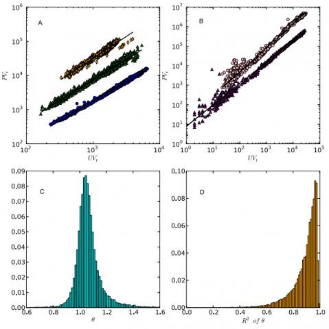
Fig. 4 (A, B) show the empirical scalings between TST and IS for five clickstream networks. In which IS denotes the number of unique users who visit the online forum or the community in one hour (day) (UV), while TST stands for the total number of clicks(or tagging activities) generated by these users in one hour (day) (PV). So θ characterizes the stickiness [33] of a forum or an online community, because, it indicates the percentage of how many visits or tagging activity will be increased when the number of users increased by 1%.
Θ for all 29,993 baidu online forms, and the distribution of the exponents and the R-squares of the scalings are shown in Fig. 4. B and C respectively. More than 86% of forums have R2>0.8 in the fitting, which suggests that the users of different forums obey similar behaviours in browsing threads collectively. Besides, 82% of the forums have a θ>1. Thus most of the studied forums are “sticky”, in the sense that users are more likely to remain in the forums when the forums grow in size.
Figure (A) The allometric growth across three forums. Data points of different forums are shown in different colours. The values of θ are 1.15 (blue circles), 1.21 (green triangles), and 1.29 (orange diamonds), respectively. (B) The allometric growth of Delicious (pink circles) and Flickr (purple triangles). Each data point corresponds to a pair of daily UV(t) and PV(t). The values of θ are 1.23 and 1.10, respectively. (C) The distribution of θ of 29,993 forums (the estimation of the rest 7 forums are removed due to a lack of data). The mean value is 1.06 and the standard deviation (SD) is 0.10. (D) The distribution of R2 in fitting the scaling of Baidu forums. The mean value is 0.89 and the SD is 0.10.
We also observed the same allometric growth patterns for other flow networks, but the results are not published yet. Therefore, we discard those results.
Figure 5.
3.2 Dissipation law
As pointed by the earlier ecological studies [16,34], a large fraction of energy flows dissipates to the environment in the whole ecosystem. The dissipated energy flow can be captured by the variable Di which is also available from the original data. Empirically, Di scales with throughflow Ti in the following way:
$D_{i} \propto c T_{i}^{\gamma}$(11)
This equation is called dissipation law in this paper, where c and γ are parameters to be estimated.
We observe that the estimated exponents γ are all slightly smaller than 1 in the energetic food webs , therefore the dissipation rate (dissipation per throughflow) decreases with the throughflow of the species slightly. If γ =1, c is the average energy dissipation rate of the whole food web. Since the empirical exponents in Table 2 are approaching to 1, the coefficient c’s are almost the dissipation rate of the specific food web.
From Table 2, we can read c’s are fractional numbers that are smaller than one except the food web Narragan whose exponent γ deviates 1 significantly.
Dissipation law is also found in other flow networks. For example, we report the pattern and the exponents in the clickstream networks of Baidu forum [27]. And we found that compare to the energetic food webs, the dissipation law exponents in clickstream networks have wider range.
Table 2. Fitting exponents and goodness of power law relationships (the webs are sorted by their number of edges, γ, α are exponents of dissipation law and gravity law. And α 1, α 2 are exponents of bi-gravity law)
|
networks |
c |
γ |
R2diss |
α |
R2gra |
α1 |
α2 |
R2bi |
|
CrystalD |
0.67 |
0.96 |
1.00 |
0.63 |
0.70 |
0.57 |
0.75 |
0.74 |
|
CrystalC |
0.68 |
0.96 |
0.99 |
0.53 |
0.65 |
0.50 |
0.57 |
0.65 |
|
ChesLower |
0.49 |
0.95 |
0.99 |
0.70 |
0.75 |
0.61 |
0.84 |
0.76 |
|
Chesapeake |
0.50 |
0.99 |
0.98 |
0.68 |
0.84 |
0.62 |
0.77 |
0.85 |
|
ChesMiddle |
0.47 |
0.88 |
0.85 |
0.67 |
0.77 |
0.60 |
0.78 |
0.78 |
|
ChesUpper |
0.58 |
0.95 |
0.99 |
0.64 |
0.64 |
0.62 |
0.67 |
0.64 |
|
Narragan |
2.05 |
0.81 |
0.94 |
0.54 |
0.81 |
0.49 |
0.60 |
0.81 |
|
Michigan |
0.67 |
0.99 |
1.00 |
0.62 |
0.86 |
0.57 |
0.72 |
0.87 |
|
StMarks |
0.43 |
0.99 |
0.95 |
0.68 |
0.74 |
0.76 |
0.56 |
0.75 |
|
Mondego |
0.53 |
0.98 |
1.00 |
0.79 |
0.85 |
0.83 |
0.70 |
0.86 |
|
Cypwet |
0.46 |
0.97 |
0.99 |
0.70 |
0.84 |
0.85 |
0.55 |
0.87 |
|
Cypdry |
0.41 |
0.96 |
0.95 |
0.68 |
0.81 |
0.81 |
0.57 |
0.83 |
|
Gramdry |
0.58 |
0.97 |
1.00 |
0.66 |
0.76 |
0.61 |
0.73 |
0.77 |
|
Gramwet |
0.59 |
0.98 |
1.00 |
0.71 |
0.81 |
0.66 |
0.79 |
0.81 |
|
Mangdry |
0.45 |
0.98 |
0.98 |
0.58 |
0.77 |
0.60 |
0.56 |
0.77 |
|
Mangwet |
0.44 |
0.98 |
0.98 |
0.59 |
0.77 |
0.60 |
0.57 |
0.77 |
|
Baywet |
0.33 |
0.92 |
0.95 |
0.62 |
0.79 |
0.67 |
0.54 |
0.80 |
|
Florida |
0.33 |
0.92 |
0.95 |
0.62 |
0.79 |
0.67 |
0.54 |
0.80 |
|
Baydry |
0.32 |
0.91 |
0.95 |
0.61 |
0.78 |
0.68 |
0.52 |
0.78 |
3.2.1 Relationship between exponents Interestingly, we further find the exponent γ of dissipation law as negative relationship with both scaling exponent η and allometric growth exponent θ.
In the energetic food web study, we simply plot ηs against γs across all the collected empirical flow networks. The result is shown in Fig. 5.
Figure 5. The relationship between γ and η in original and adjusted ecological flow networks
In Fig. 5, the blue dotted curve is the original flow network, and the solid red line is for the adjusted networks based on the same network structure and the dissipation law according to flow adjusted algorithm (based on the Mondego’s topology but assigning flows randomly) [36]. We observe the allometric scaling exponent decreases with the dissipation law exponent in a similar manner no matter the original network structures are.
Figure 6. The negative correlation between γ and θ. We plot both of the linear-binned data (orange circles) and the original data (heat map)
Another interesting phenomenon that we noticed in the research of clickstream networks is that the dissipation efficiency γ and the allometric exponent θ are related. A small γ indicates when a node’s through-flow increases, the dissipation rate may decrease and thus increase the network storage capacity. Fig. 6. demonstrates that the empirical data support the negative correlation between them.
So, we suppose the reversed chronological displaying order of threads seems to decrease the dissipation efficiency γ and increase the ‘‘stickiness’’ θ of the studied forums. This may be the reason why such displaying order is so common among forums. The web masters may or may not have noticed that, this strategy beats its competitors by generating flow structure that attracts more users and thus spreads out in the evolution of forums.
In summary, the dissipation index γ is very significant in the open flow networks. It can not only connect with allometric laws, but also may determine other important network properties, such as robustness, the efficiency of transportation and the growth of the network.
3.3 Gravity law
Another important common pattern found in flow networks is called gravity. It depicts the relationship between the flux on edges and nodes.
We confirm this pattern in energetic food webs. We actually uncovered that the large throughflow nodes can exchange large energy flows. This effect is reflected by the so-called gravity law, namely, the energy flow between i and j scales with the product of the total throughflows of i and j, i.e.
$f_{i j} \propto\left(T_{i} T_{j}\right)^{\alpha}$(12)
In the case of food webs, the throughflow of each node Ti is treated as the size of a node comparable to the population of a city. It has similar forum as the famous Newton’s gravity law in which Ti and Tj are treated of two nodes, and the flux fij is treated as the force between the two. However, the distance d has no correspondence because spatial information is not included in our energetic food webs.
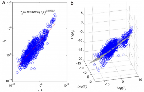
Fig. 7. shows this pattern for a specific food web as an example. And all the results of exponents for all the food webs we have collected are shown in the fourth column of Table 2.
Figure 7. Univariate and bivariate gravity law of Mangwet food web(a); The bivariate scaling relationship
From Fig. 7(a), we could observe that there are several straight bands in the clusters of data points which indicate that the energy flow between two nodes fij may be predicted by other variables rather than the product of Ti and Tj .
In order to fit better with the real data, we suggest that the following bivariate scaling relation holds:
$f_{i j} \propto T_{i}^{\alpha 1} T_{j}^{\alpha 2}$(13)
Where α1 and α2 are two estimated parameters. This form of gravity law implies that the start nodes and the end nodes are asymmetric in the flow networks. Fig. 7(b) shows this bivariate gravity law. All the estimated exponents α1 and α2 and the corresponding R2 are shown in the last 2nd, 3rd and 4th columns in Table2. We can observe from Table 2 that the exponent α2 is larger than α1 for small food webs but smaller than it for large food webs except Gramdry and Gramwet. Thus, we can conclude that the large energy flows prefer to link nodes with large throughflow in all energy flow networks.
All of these observed patterns of energy flows exhibit statistical significance and universality for all 19 empirical food flow networks and this scaling relation is also exists in other open flow systems like traffic flow networks or trade flow networks and so on.
A basic principle in all flow systems first proposed by the famous scientist Bejan. It claims that the generation of images of design in nature is a phenomenon of physics and this phenomenon is covered by the principle that all systems evolve in such a way that they provide easier access to flow [35].
Until now this principle has been widely applied from river networks, meridian networks to the animal behaviour networks. Consequently, it is reasonable to suppose that the general open flow networks may also obey this law in the process of evolution.
To quantify this law in the framework of flow networks, the first thing we should do is to formulate it and to figure out what does easier access to flow mean for flow networks.
Two important quantities will be defined in advance. they are the flow distance Lij and the total flux Tij. Here, the flow distance Lij is defined as the average steps that a particle flow from node i to j on all paths(directed and indirected) , it can be calculated by the following equation:
$L_{i j}=\frac{\left(M U^{2}\right)_{i j}}{u_{i j}}-\frac{\left(M U^{2}\right)_{j j}}{u_{j j}}$(14)
M, U are the matrices introduced in the section 2.
Similarly, the total flows Tij is defined by the total flux from i to j along all possible paths (directed and indirected), which can be expressed
$T_{i j}=f_{0} \frac{u_{0 i}}{u_{i i}} u_{i j}$(15)
Where, u and f are the elements in matrix U and F.
If the constructal law holds for open flow networks, then the flows may access the system easier means that the flow distance between any two nodes i and j will become shorter, and the total flows between them will become larger as the network evolve. This is the formulation of the constructal law in flow networks.
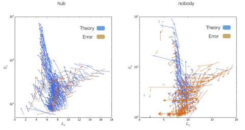
Next, we will test this hypothesis by evolving clickstream networks (Baidu online forum). First, for each node i in the network as a reference, at any time t, we can plot two variables Tij and Lij for any other node j on a plot (shown in Fig. 8). While under the evolution, after a period of time, there is another corresponding pair: T’ij and L’ij for the same node pair. We draw both of them on the picture and marked the direction from (Lij , Tij) to (L’ij , T’ij). Second, we color the directions that are consistent with the constructal law blue, and other directions as yellow. All these directions are pointing up or left because according to the formulation of constructal law, the distances will be shorter and the total flux will be larger. In Fig. 8, we show arrows for two representative nodes as references: a hub (left) and a nobody(left).
Figure 8. The changes of Tij and Lij in the study on EXO forum. The time interval is about 2 hours
From Fig. 8, we know the hub node is consistent with the law, meaning that L’ij is smaller than Lij or T’ij is greater than Tij or both happened. However, It seems that the nobody nodes not obey the constructal law. Because hubs always dominate large flows, they have large weights, thus the constructal law is approximately hold for the entire network.
The underlying reasons behind these phenomena are still not clear. In the study of allometric law, an interesting and still unexplained finding is that the allometric exponents of empirical ecological networks are all close to 1. They are neither centralized nor decentralized. We conjecture that this finding can be explained by an optimization between flow structure stability and energy transport efficiency, but this hypothesis will require additional study.
Moreover, although the constructal law can be formulated by the conceptions of flow distances and total flows, more empirical studies on flow network evolution are needed. The results in this paper are very rough to make some scientific conclusion. However this is the first step which is meaningful.
1. M. Newman, A.L. Barabasi, and D.J., Watts, “The structure and dynamics of networks,” Princeton University Press, 2006.
2. A. L. Barabasi and E. Bonabeau, “Scale-Free netwroks,” Scientific American, 50, 2003.
3. S.H. Strogatz, “Exploring complex networks,” Nature 410(6825), 268-276, 2001. DOI: 10.1038/35065725.
4. R. Albert and A.L. Barabasi, “Statistical mechanics of complex networks,” Reviews of Modern Physics 74, 47-97, 2002. DOI: 10.1103/RevModPhys.74.47.
5. A. Barrat, M. Barthelemy, R. Pastor-Satorras, and A. Vespignani, “The architecture of complex weighted networks,” Proceedings of the national academy of sciences, 101 (11), 3747-3752, 2004. DOI: 10.1073/pnas.0400087101.
6. S. Horvath, “Weighted network analysis,” Applications in Genomics and Systems Biology, Springer, 2011. DOI: 10.1007/978-1-4419-8819-5.
7. A.S. Asratian, T.M.J. Denley, and R. Haggkvist, Bi-Partite Graphs and Their Applications, Cambridge University Press, 1998.
8. P. Holme and J. Saramaki, “Temporal networks,” Physics Reports, 19 (4), 532-538, 2012. DOI: 10.1016/j.physrep.2012.03.001.
9. G. Nicolis and P. Ilya, “Self-organization in nonequilibrium systems,” Wiley, New York, 1977.
10. G.B. West and J. Brown, “The origin of allometric scaling laws in biology from genomes to ecosystems: towards a quantitative unifying theory of biological structure and organization,” Journal of Experimental Biology, 208 (9), 1575-1592, 2005. DOI: 10.1242/jeb.01589.
11. J. Banavar, A. Maritan, and A. Rinaldo, “Size and form in efficient transportation networks,” Nature, 399 (6732), 130-132, 1999.
12. M. Higashi, “Extended input-output flow analysis of ecosystems,” Ecological Modelling, 32, 137-147, 1986. DOI: 10.1016/0304-3800(86)90022-0.
13. W. Leontief, The Structure of American Economy, Harvard University Press, 1941.
14. W. Leontief, Input-output Economics, Oxford University Press, 1986. DOI: 10.1038/scientificamerican1051-15.
15. R.E. Miller and P.D. Blair, Input-Output Analysis: Foundations and Extensions, Cambridge University Press, 2009. DOI: 10.1017/CBO9780511626982.
16. H. Odum, System Ecology: An Introduction, John Wiley & Sons Inc, 1983.
17. H.T. Odum, “Slef-organization, transformity, and information,” Science, 242, 1132-1139, 1988.
18. R.E. Ulanowicz, Ecology, the Ascendent Perspective, Columbia University Press, 1997.
19. R.E. Ulanowicz, “Quantitative methods for ecological network analysis,” Computational Biology and Chemmistry, 28 (5), 321-339, 2004. DOI: 10.1016/j.compbiolchem.2004.09.001.
20. J. Zhang and L. Guo, J., “Scaling behaviours of weighted food webs as energy transportation networks,” Journal of Theoretical Biology, 264 (3), 760-770, 2010.
21. J. Zhang and L. Wu, “Allometry and dissipation of ecological flow networks,” PLoS ONE, 8 (9), e72525, 2013. DOI: 10.1371/journal.pone.0072525.
22. J. Zhang and Y. Feng, “Common patterns of energy flow and biomass distribution on weighted food web,” Physica, A 405, 278-288, 2014. DOI: 10.1016/j.physa.2014.03.040.
23. B.D. Fath and B.C. Patten, “Review of the foundations of network environ analysis,” Ecosystems, 2, 167-179, 1999. DOI: 10.1007/s100219900067.
24. J.T. Finn, “Measures of ecosystem structure and function derived from an analysis of flow,” Journal of Theoretical Biology, 56, 363-380, 1976. DOI: 10.1016/S0022-5193(76)80080-X.
25. M. Higashi, B.C. Patten, and T.P. Burns, “Network trophic dynamics: the modes of energy utilization in ecosystems,” Ecological Modelling, 66, 1-42, 1993. DOI: 10.1016/0304-3800(93)90037-S.
26. S. Levine, “Several measures of trophic structure applicable to complex food webs,” Journal of Theoretical Biology, 83, 195-207, 1980. DOI: 10.1016/0022-5193(80)90288-X.
27. L. Wu, J. Zhang, and M. Zhao, “The metabolism and growth of web forums,” PLoS ONE, 9 (8), e102646, 2014. DOI: 10.1371/journal.pone.0102646.
28. L. Wu and J. Zhang, “The decentralized flow structure of clickstreams on the web,” European Physics Journal, B 86 (6), 1-6, 2013. DOI: 10.1140/epjb/e2013-40132-2.
29. P. Shi, J. Zhang, and J. Luo, “Hierarchicality of trade flow networks reveals complexity of products,” PLoS ONE, 9 (6), e98247, 2014. DOI: 10.1371/journal.pone.0098247.
30. S. Vitali, J.B. Glattfelder, S. Battiston, “The network of global corporate control,” PLoS ONE, 6, e25995, 2011. DOI: 10.1371/journal.pone.0025995.
31. D. Garlaschelli, G. Caldarelli and L. Pietronero, “Universal scaling relations in food webs,” Nature, 423, 165-168, 2003. DOI: 10.1038/nature01604.
32. G.B. West, J.H. Brown and B.J. Enquist, “A general model for the origin of allometric scaling laws in biology,” Science, 276: 122–126, 1997. DOI: 10.1126/science.276.5309.122.
33. R.E. Bucklin, J.M. Lattin, A. Ansari, S. Gupta, “Choice and the internet: from clickstream to research stream,” Marketing Letters, 13, 245–258, 2002.
34. R.L. Lindeman, “The trophic-dynamic aspect of ecology,” Ecology, 23, 399–418, 1942. DOI: 10.2307/1930126.
35. Adrian Bejan and Sylvie Lorente, “The constructal law of design and evolution in nature,” Philosophical Transactions of the Royal Society, B 365, 1135-1347, 2010. DOI: 10.1098/rstb.2009.0302.
36. R.J. Williams and N. Martinez, “Simple rules yield complex food webs,” Nature, 404, 180–183, 2000. DOI: 10.1038/35004572.