OPEN ACCESS
In order to study the flow, bed deformation and sediment transportation in Daliushu Reach of the Yellow River, a threedimensional (3D) turbulence model under body-fitted coordinates is developed and the flow condition in the continuous bends in the Daliushu Reach is numerically simulated. Finite volume method under unstructured grids is used to discretize the governing equations, and the SIMPLE algorithm is used to deal with the coupled problem of pressure and velocity. The numerical result is verified with the experimental data field measured from October 2010 to November 2011. The consistence between the simulated and measured longitudinal and transverse velocities indicated that the model can reasonably simulate the flow movement in continuous bends of the Yellow River. The numerical results are beneficial to the construction of the Daliushu Water Control Project.
3D turbulence model; finite volume method; numerical simulation; Daliushu Reach of the Yellow River.
Continuous bends are common in natural rivers and have been intensively studied in the past decades. The study of river flow in bends plays an important role in many areas of hydraulic engineering and the research results have been widely applied in river management, port construction, water diversion, sediment prevention and waterway improvement, etc. The Yellow River is a world-famous high sediment river with continuous bends. When the discharge is large, the flow direction in the Yellow River is toward to straight line. However, when the discharge is small, the water will flow along the bends of the river. The Daliushu Reach of the Yellow River is located at the exit of the Heishan Gorge near the junction of Ningxia Hui Autonomous Region and Gansu Province. The studied reach is an alluvial plain river that is mainly affected by upstream water and sediment. In the Daliushu Reach, less water carries large amount sediment, with different sources. Moreover, most of water and sediment in the studied reach come from flood season. In the past two decades, due to some reasons such as significant decrease of upstream runoff, the discharge and sediment capacity have been reduced. Therefore, the water and sediment loosed balance, and the river bed has been deposited severely. The river bed becomes wide, shallow, wandering and disordered. As a result, the flood discharge capacity was reduced greatly.
Wilson (2003), Validation of a three-dimensional (3D) finite volume code solving the Navier–Stokes equations with the standard k-epsilon turbulence model is conducted using a high quality and high spatial resolution data set. Zhang et al. (2007) analyzed the 3D RNG $k-\varepsilon$ turbulence hydrodynamic model in non-orthogonal curvilinear coordinates and simulated two examples of the meandering channel and Fall River. Zhong et al. (2009) studied the 2D numerical model of flow and sediment for wandering rivers and simulated the collapse of river bank. Abhari (2010) studied the flow pattern in a 90° bend experimentally and numerically. Jennifer (2010) studied 2-D depth-averaged hydrodynamic model to simulate the evolution of meandering channels from the complex interaction between downstream and secondary flows, bed load and suspended sediment transport, and bank erosion. Zhou et el.(2010) and Yi et al.(2010) established 2D mathematical model including the effect of secondary flow of river bend and bank collapse and verified the measured data of laboratory flume experiments. JIA et al.(2010,2011) provided a method to calculate equivalent making channel discharge for alluvial river with obvious bank collapse and bed deformation and conducted 3D numerically simulation for the flow and sediment of Shishou Reach in Jingjiang river. Hu et al. (2011) studied the influence of transition section in continuous bend. Song et al. (2011) studied unstructured finite volume model to simulated dam-break flow with complex boundry. Lv et al. (2013) analyzed the measured data in Daliushu Reach of the Yellow River. Zhao et al. (2013) analyzed 3D the realizable $k-\varepsilon$ turbulence model and solved the governing equations by the finite volume method, and to simulate the flow field around fishing plane nets. Petr et al. (2014) applied the finite volume and finite element method to simulated incompressible turbulent flow over the backward facing step with various inclinations. Huang et al. (2014) established 3D numerical model to simulate the flow around the water intake in the natural river, based on the RANS equations and $k-\varepsilon$ turbulent model.
With the development of computer technology, 3D turbulence models of flow and sediment are valued and applied in the field of hydraulic engineering. However, research results about 3D numerical simulation of flow in Daliushu Reach in the Yellow River are still very few. In this paper, a revised 3D $k-\varepsilon$ turbulence model based on unstructural grid was used to simulate the flow of Daliushu Reach in the Yellow River. The data of the reach measured from October 2010 to November 2011 was used to verify the mathematical model. The flow in the studied reach is numerically simulated, which is beneficial to understand the flow characteristics. Furthermore, the research results are helpful to the construction and management of the Daliushu Water Control Project that will be built in the near future.
2.1 The governing equations
Since the flow in the studied reach is obvious turbulent, so a turbulence model named as revised $k-\varepsilon$ model [12] is adopted to numerically simulate the flow in Daliushu Reach. The three-dimensional governing equations in the Cartesian coordinate system are as followings.
Continuity equation,
$\frac{\partial u_{i}}{\partial x_{i}}=0$ (1)
where $x_{i}(i=1,2,3)$ are the coordinates in the Cartesian coordinate system, $u_{i}(i=1,2,3)$ are the velocity components.
Momentum equation,
$\frac{\partial u_{i}}{\partial t}+\frac{\partial}{\partial x_{j}}\left(u_{i} u_{j}\right)=\frac{\partial}{\partial x_{j}}\left(\left(v+v_{t}\right) \frac{\partial u_{i}}{\partial x_{j}}\right)-\frac{1}{\rho} \frac{\partial p}{\partial x_{i}}+g_{i}$ (2)
in which $i, j=1,2,3$ indicate the Cartesian coordinates $(x, y, z)$, $t$ is the time, $v$ is the coefficient of kinematic viscosity of water, $p$ is time averaged hydrodynamic pressure, $\rho$ is the density of water, $g_{i}$ are components of the gravitational acceleration in three coordinate directions, $V_{t}$ is the sports eddy viscosity coefficient,
$v_{t}=C_{\mu} \frac{k^{2}}{\varepsilon}$ (3)
$k$- and $\varepsilon$ - equations,
$\frac{\partial k}{\partial t}+\frac{\partial}{\partial x_{j}}\left(k u_{j}\right)=\frac{\partial}{\partial x_{j}}\left(\left(v+\frac{v_{t}}{\sigma_{k}}\right) \frac{\partial k}{\partial x_{j}}\right)+G_{k}-\varepsilon$ (4)
$\frac{\partial \varepsilon}{\partial t}+\frac{\partial}{\partial x_{j}}\left(\varepsilon u_{j}\right)=\frac{\partial}{\partial x_{j}}\left(\left(v+\frac{v_{t}}{\sigma_{\varepsilon}}\right) \frac{\partial \varepsilon}{\partial x_{j}}\right)+C_{1} S \varepsilon-C_{2} \frac{\varepsilon^{2}}{k+\sqrt{v \varepsilon}}$ (5)
where $k$ is the turbulent energy,$\mathcal{E}$ is turbulent energy dissipation rate, $G_{k}$ is a production term caused by the average velocity gradient of the turbulent kinetic energy, $S$ is time averaged strain rate tensor,
$G_{k}=2 v_{t} S_{i j} S_{i j}$ (6)
$S=\sqrt{2 S_{i j} S_{i j}}$ (7)
$S_{i j}=\frac{1}{2}\left(\frac{\partial u_{i}}{\partial x_{j}}+\frac{\partial u_{j}}{\partial x_{i}}\right)$ (8)
$\sigma_{k}$ and $\sigma_{\varepsilon}$, respectively, represent the turbulent kinetic energy and the dissipation rate Prandtl number, in this place,$\sigma_{k}=1.0, \sigma_{\varepsilon}=1.2, C_{1}=1.7, C_{2}=1.9, C_{\mu}=0.0845$
2.2 The turbulence model of flow in body-fitted coordinates
The banks of natural rivers are usually irregular and the river beds are very complex. Therefore, it is necessary to transform equations (1)-(5) to body-fitted coordinates [12]. The generalized form is as followings,
$\frac{\partial \Phi}{\partial t}+\frac{\partial}{\partial \xi}(U \Phi)+\frac{\partial}{\partial \eta}(V \Phi)+\frac{\partial}{\partial \zeta}(W \Phi)=\frac{\partial}{\partial \xi}\left(A \Gamma_{\Phi} \frac{\partial \Phi}{\partial \xi}\right)+\frac{\partial}{\partial \eta}\left(B \Gamma_{\Phi} \frac{\partial \Phi}{\partial \eta}\right)+\frac{\partial}{\partial \zeta}\left(C \Gamma_{\Phi} \frac{\partial \Phi}{\partial \zeta}\right)+S_{\Phi}(\xi, \eta, \zeta)$ (9)
Where
$U=u \xi_{x}+v \xi_{y}, V=u \eta_{x}+v \eta_{y}$
$W=u \zeta_{x}+v \zeta_{y}+w \zeta_{z}$
$A=\xi_{x}^{2}+\xi_{y}^{2}, B=\eta_{x}^{2}+\eta_{y}^{2}$
$C=\zeta_{x}^{2}+\zeta_{y}^{2}+\zeta_{z}^{2}$
in which $\xi_{x}, \xi_{y}, \xi_{z}$ are the respectively derivatives of the $\xi$ in $x, y, z$ direction, $\eta_{x}, \eta_{y}, \eta_{z}$ are the respectively derivatives of the $\eta$ in $x, y, z$ direction , $\zeta_{x}, \zeta_{y}, \zeta_{z}$ are the respectively derivatives of the $\zeta$ in $x, y, z$ direction , $\Phi$ is the common variable, may represent $1, u_{1}, u_{2}, u_{3}, k, \varepsilon$ , $\Gamma_{\Phi}$ is the coefficient of diffusion, $S_{\Phi}$ is the source item, their meanings are shown in Table 1.
Table 1. Some variables and coefficients in the body-fitted coordinates
|
$\Phi$ |
$\Gamma_{\Phi}$ |
$S_{\Phi}$ |
|
|
Continuity equation |
1 |
0 |
0 |
|
$x-$momentum equation |
$u_{1}$ |
$v+v_{t}$ |
$S_{u 0}+S_{u 1}$ |
|
$y-$momentum equation |
$u_{2}$ |
$v+v_{t}$ |
$S_{v 0}+S_{v 1}$ |
|
$z-$momentum equation |
$u_{3}$ |
$v+v_{t}$ |
$S_{w 0}+S_{w 1}$ |
|
$k$ equation |
$k$ |
$v+v_{t} / \sigma_{k}$ |
$S_{k 0}+S_{k 1}$ |
|
$\varepsilon$ equation |
$\varepsilon$ |
$v+v_{t} / \sigma_{\varepsilon}$ |
$S_{\varepsilon 0}+S_{\varepsilon 1}$ |
in which:
$S_{u 0}=-\frac{1}{\rho} \frac{\partial p}{\partial x}=-\frac{1}{\rho}\left(\frac{\partial p}{\partial \xi} \xi_{x}+\frac{\partial p}{\partial \eta} \eta_{x}+\frac{\partial p}{\partial \zeta} \zeta_{x}\right)$ (10)
$S_{v 0}=-\frac{1}{\rho} \frac{\partial p}{\partial y}=-\frac{1}{\rho}\left(\frac{\partial p}{\partial \xi} \xi_{y}+\frac{\partial p}{\partial \eta} \eta_{y}+\frac{\partial p}{\partial \zeta} \zeta_{y}\right)$ (11)
$S_{w 0}=-\frac{1}{\rho} \frac{\partial p}{\partial z}-g=-\frac{1}{\rho} \frac{\partial p}{\partial \zeta} \zeta_{z}-g$ (12)
$S_{k 0}=G_{k}-\varepsilon, S_{\varepsilon 0}=C_{1} S \varepsilon-C_{2} \frac{\varepsilon^{2}}{k+\sqrt{v \varepsilon}}$ (13)
$S_{\Phi 1}=\frac{\partial}{\partial \xi}\left[\left(\xi_{x} \eta_{x}+\xi_{y} \eta_{y}\right) \Gamma_{\Phi} \Phi_{\eta}+\left(\xi_{x} \zeta_{x}+\xi_{y} \zeta_{y}\right) \Gamma_{\Phi} \Phi_{\zeta}\right]+$
$\frac{\partial}{\partial \eta}\left[\left(\zeta_{x} \eta_{x}+\zeta_{y} \eta_{y}\right) \Gamma_{\Phi} \Phi_{\zeta}+\left(\xi_{x} \eta_{x}+\xi_{y} \eta_{y}\right) \Gamma_{\Phi} \Phi_{\xi}\right]+$
$\frac{\partial}{\partial \zeta}\left[\left(\zeta_{x} \xi_{x}+\zeta_{y} \xi_{y}\right) \Gamma_{\Phi} \Phi_{\xi}+\left(\eta_{x} \zeta_{x}+\eta_{y} \zeta_{y}\right) \Gamma_{\Phi} \Phi_{\eta}\right]$ (14)
3.1 Computational area and mesh generation
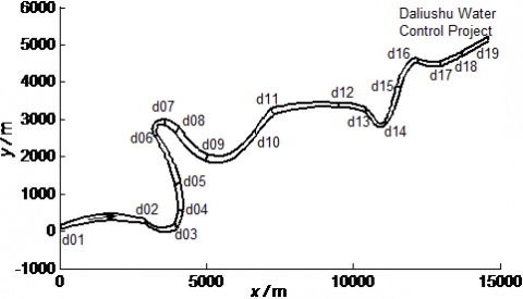
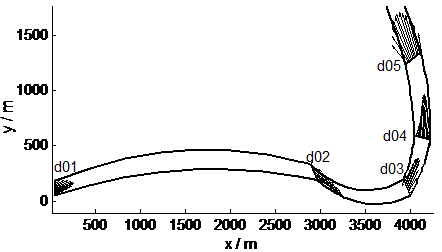
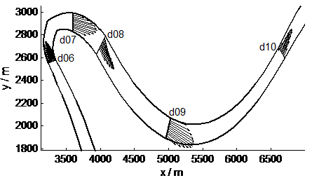
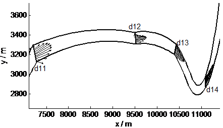
The Daliushu Reach in the Yellow River in this study is about 20km, and the averaged width is 143.11m. The discharge is 903m3/s. The water level at the inlet is 1256.32m, and it is 1242.40m at the outlet. The studied reach is shown in Fig.1. Nineteen cross-sections are arranged for field measuring.
Figure 1. The layout of Daliushu river section
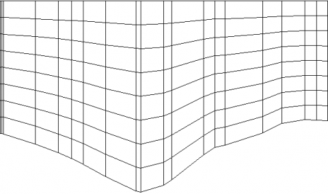
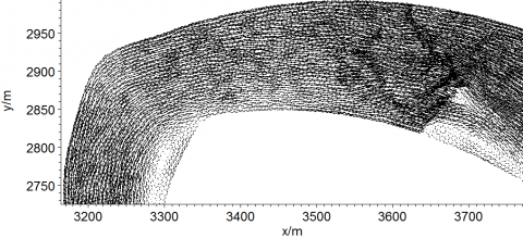
Unstructured mesh is used for the study area, and various mesh densities are adopted according to actual requirement considering the computation precision and time consumption. There are 430344 grid nodes in the computation area and the time step is 2s. Because the studied reach is very long, the mesh of full region is quite complicated. Therefore, some part of the studied area is enlarged, as shown in Fig. 2.
(a) Transverse cross section in d10
(b) Plane
Figure 2. Local meshes in Daliushu Reach from d13 to d15
3.2 Boundary conditions
Boundary conditions include conditions at inlet, outlet, solid wall and free surface, respectively.
At inlet boundary, discharge is given as $Q=903$ m3/s, $k$ and $\varepsilon$ are calculated by [16],
$k=0.00375\left(u_{1}^{2}+u_{2}^{2}\right), \varepsilon=0.09 k^{3 / 2} /(0.05 h)$ (15)
where $u_{1}$ and $u_{2}$ are the respectively velocity in $x$, $y$ direction, and given by measured. $h$ is water depth at inlet.
At outlet boundary, water level is presented as $z=1242.40$ m, and other variables are dealt with full developed boundary conditions,
$\frac{\partial \Phi}{\partial z}=0$ (16)
in which $\Phi$ is the common variable, may represent $u_{1}, u_{2}, u_{3}, p, k, \varepsilon$.
At solid wall boundary, no slip condition is adopted and dealt with wall function method [17].
At free surface boundary, water level of calculated nodes are given by the interpolation of measured water level, and the rigid lid assumption is used.
$\frac{\partial \Phi}{\partial z}=0, u_{3}=0$ (17)
in which $\Phi$ is represent $u_{1}, u_{2}, p, k, \varepsilon$.
3.3 Numerical methods
The 3D coordinate transformation is used to transform the irregular physical area to regular computation area, and the governing equations are also transformed to new equations in the body-fitted coordinates. Finite volume method is applied to discrete the governing equation in the computation area. The central difference scheme is used to discrete the diffusion and source terms.The QUICK scheme is used to discrete the convection term. The SIMPLE algorithm is used to deal with the coupled problem of pressure and velocity.
The field measured data in November 2011 were used to verify the flow model and to set the initial conditions for the studied reach. Advanced instruments such as River CAT, Echo Sounder, 3D laser scanner were carried to measure river bed elevation, velocity, river width and water level on the 19 typical cross sections in Daliushu Reach of the Yellow River. Some basic data of these cross-sections are shown in Table 2, in which the left bank of the first river bend (from d02 to d05) is convex bank, while the right bank is concave bank. Water level is higher near the concave bank (right bank) than that near the convex bank (left bank). The transverse gradient of water surface in the second bend (from d06 to d08) is similar to the first bend, and the water level is higher near the concave bank (left bank) than that near the convex bank (right bank). The cross surface of the water exists surface ultrahigh, it forms the transverse gradient.
Table 2. Field measured data on typical cross-sections
|
Section number |
Water level of left bank (m) |
Water level of right bank (m) |
Averaged water depth (m) |
Width of river (m) |
Averaged velocity (m/s) |
|
d01 |
1258.36 |
1258.39 |
5.02 |
101.7 |
1.64 |
|
d02 |
1255.90 |
1255.95 |
2.98 |
161.1 |
1.72 |
|
d03 |
1253.81 |
1254.04 |
3.80 |
138 |
1.8 |
|
d04 |
1253.50 |
1253.53 |
3.81 |
175.8 |
1.22 |
|
d05 |
1252.53 |
1252.95 |
2.47 |
195.8 |
1.49 |
|
d06 |
1251.14 |
1251.00 |
4.25 |
101.5 |
1.82 |
|
d07 |
1250.80 |
1250.70 |
3.25 |
157.2 |
1.93 |
|
d08 |
1250.18 |
1250.15 |
3.0 |
228.3 |
1.23 |
|
d09 |
1249.32 |
1249.47 |
2.64 |
184 |
1.98 |
|
d10 |
1248.13 |
1248.11 |
3.81 |
117.9 |
1.83 |
|
d11 |
1247.88 |
1247.80 |
5.37 |
171.8 |
1.1 |
|
d12 |
1246.60 |
1246.56 |
5.32 |
123.3 |
1.82 |
|
d13 |
1246.29 |
1246.24 |
5.39 |
109.7 |
2.06 |
|
d14 |
1246.02 |
1246.11 |
4.73 |
111.8 |
1.87 |
|
d15 |
1244.95 |
1244.88 |
3.32 |
134.7 |
1.75 |
|
d16 |
1244.02 |
1243.52 |
4.26 |
132.7 |
1.9 |
|
d17 |
1243.49 |
1243.61 |
4.29 |
137.3 |
1.74 |
|
d18 |
1242.99 |
1242.99 |
5.11 |
100.4 |
2.14 |
|
d19 |
1242.40 |
1242.32 |
4.65 |
136 |
1.76 |
4.1 Analysis of water level
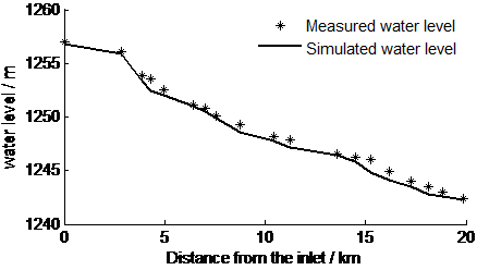
The comparison between the measured and simulated water level at the river center line is shown by Figure 3, where the horizontal axis is the distance from the inlet, and the vertical axis is the water level of free surface. From Figure 3, it can be found that the measured and simulated water levels are in good agreement and they both decrease from upstream to downstream.
Figure 3. Comparison of water level between simulated and measured results
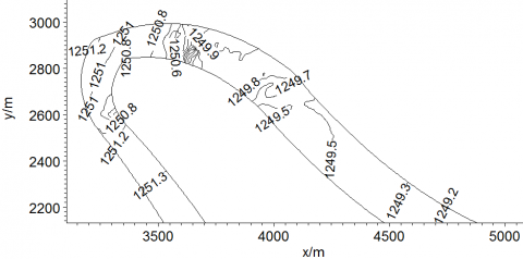
The contour line of water level from d06 to d08 is shown by Figure 4. It can be found the water level at concave bank (1251.2m) is higher than that at convex bank (1250.8m), which is consistent with the general rule in a bend of rivers. Therefore, the turbulence model in this paper can accurately simulate the water level of free surface and physical phenomenon in a bend of rivers.
Figure 4. Contour line of water level in bend of studied reach from d06 to d08
4.2 Analysis of water flow field
The measured flow field in the studied reach is shown in Figure 5(a) to Figure 5(d), where the discharge at inlet is 903m3/s.
(a) Measured flow field from d01 to d05
(b) Measured flow field from d06 to d10
(c) Measured flow field from d11 to d14
(d) Measured flow field from d15 to d19
Figure 5. Measured flow field in Daliushu Reach of the Yellow River
Figure 5 shows the sections d02, d03 and d04 are located at inlet, curved top and outlet in the first bend, respectively. Due to the effect of upstream bend, the water flow has not been fully developed. The maximum velocity appears near the convex bank at the first bend such as d02 and d03. The velocity near the convex bank is greater than that of the concave bank. At section d04, the maximum velocity appears near the concave bank. The section d05 is located at the transition section between the first and second bends. Because the transition part is long enough, the flow from the first bend is developed fully. Sections d06, d07 and d08 are located at inlet, curved top and outlet in the second bend, respectively. At inlet of the second bend (d06), the maximum velocity begin to transit to the concave bank. At the bend top (d07), the maximum velocity appears near the concave bank. At outlet of the bend (d08), the bend flow has been fully developed, where the mainstream appears the center of river. Therefore, the flow distribution of continuous bend is not only affected by the discharge, but also affected by the upstream bend.
The flow field distribution of sections d15 to d19 are stable, and the mainstream distribute at the center of river basically.
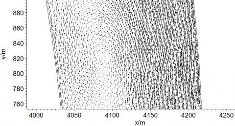
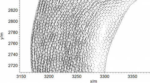
The simulated flow field in the studied reach is shown in Figure 6.The simulated flow field in the area from d06 to d08 is shown in Figure 6(a), in which the mesh grid is relatively finer. Similarly, the simulated flow field in the area from d13 to d15 is shown in Figure 6(b), in which the mesh grid is relatively less fine than that in Figure 6(a). It can be seen in above figures that the actual flow field can be simulated more accurately when the mesh grid is fine. However, if the grid is too fine, it will cost a lot of computation time. Various mesh grid scale are set at the studied reach to save computation time and to improve the convergence of the algorithm.
(a) Simulated flow field from d06 to d08
(b) Simulated flow field from d13 to d15
(c) Simulated flow field near d04
(d) Simulated flow field near d06
Figure 6. Simulated flow field in Daliushu Reach of the Yellow River
From Figure 6, it can be found that the simulated and measured velocities have similar trend, and the 3D numerical model can numerically simulated the flow field in the studied reach. The distribution of flow velocities at the first (Figure 6(c)) and second (Figure 6(d)) bends are similar. The velocity near the concave bank is greater than that of the convex bank, and surface circulation can be found near the convex bank clearly. It follows the general rules of natural curved river: the concave bank is eroded while thee convex bank is deposited.
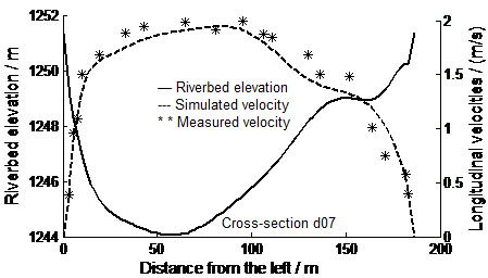
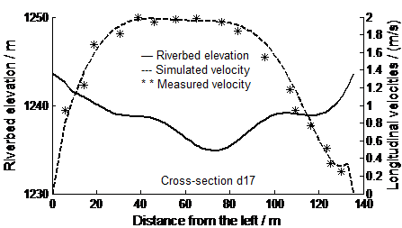
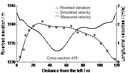
In Figure 7, the simulated and measured longitudinal mean velocities are compared on four cross-sections such as d04, d07, d17 and d18.
Figure 7. Comparison of velocities between measured and simulated results
As can be seen in Figure 7, the simulated and the measured longitudinal velocities are very close. The velocity is larger in the riverbed at the thalweg. The revised 3D![]() turbulence model can simulate the flow of continuous curve in the studied reach very well.
turbulence model can simulate the flow of continuous curve in the studied reach very well.
The cross-sections d17 and d18 are located at the dam of Daliushu hydraulic project. As can be seen from the riverbed elevation and velocity distribution , the reach composed by canyon, and the riverbed type form “V”, where the velocity distribution are stable. It shows that it is a good site to build a high dam in the Daliushu Reach of the Yellow River
4.3 The longitudinal velocity distribution in vertical direction
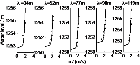
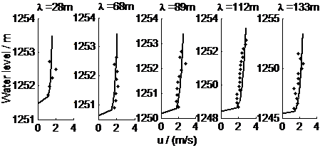
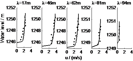
Figure 8 shows the simulated and measured longitudinal velocities are compared at five vertical lines on six typical cross-sections from d02 to d07. The first bend starts from d02 and ends at d04, where the left bank is convex bank and the right bank is concave bank. The second bend is from d06 to d08, where the left bank is concave bank and the right bank is convex bank. The cross-section d05 is located at the transition between the first and second bends. On cross-section d02, λ=34m,52m, 77m, 98m, 119m which are the distances from the left bank of five vertical lines. On cross-section d03, λ=10m, 33m, 59m, 79m, 98m which are the distances from the left bank of five vertical lines. On cross-section d04, λ=28m, 68m, 89m, 112m, 133m which are the distances from the left bank of five vertical lines. On cross-section d05, λ=27m, 58m, 84m, 113m, 164m which are the distances from the left bank of five vertical lines. On cross-section d06, λ=17m, 46m, 62m, 81m, 94m which are the distances from the left bank of five vertical lines. On cross-section d07, λ=17m, 50m, 79m, 111m, 138m which are the distances from the left bank of five vertical lines. The x-axis is the longitudinal velocity, and the y-axis is the water level.
(a) Cross-section d02
(b) Cross-section d03
(c) Cross-section d04
(d) Cross-section d05
(e) Cross-section d06
(f) Cross-section d07
Figure 8. The longitudinal velocity distribution in vertical direction
(*measured value, — simulated value)
As can be seen in Figure 8, the simulated and the measured longitudinal velocities are very close, which reflects the general rule of flow in a bend of natural rivers. After the water enters the first bend (d02-d04), the maximum is near the convex bank at the apex of the bend, and it gradually turns to the concave bank. Because the transition part between the first and second bends is long enough, the flow from the first bend is devoted fully. Therefore, the velocity distribution is close to uniform. The velocity distribution at the second bend (d06-d07) is similar to the first bend.
4.4 The distribution of transverse velocity
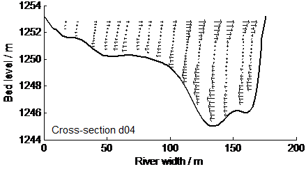
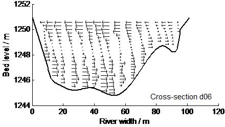
In a bend of rivers, because of the centrifugal force, the water near free surface flows from the convex bank to the concave bank, while the water near river bed flows in the opposite direction. The secondary flow on cross-section d04, d05 and d06 are shown in Figure 9, where the x-axis is the distance from the left bank, and the y-axis is the water level.
The left and right banks are convex and concave banks, respectively on cross-section d04, where the water flows towards to the concave bank near water surface and it flows towards to the convex bank near river bottom. The cross-section d05 is located at the transition section and it circulation intensity is weakened. Circulation direction begin to transform to the opposite direction. Cross-section d06 is different from d04, i.e. the left and right banks are concave and convex banks, respectively. But the secondary current on d06 is similar to d04. The water on d06 flows towards to the concave bank near water surface and it flows towards to the convex bank near river bottom. The secondary currents on d04 and d06 are accord with the general rule of flow in a river bend.
Figure 9. Transverse velocity on two typical cross-sections
It can be found in Figure 9 that the transverse velocity is approach to zero at a certain water level, and it gradually increases towards water surface and river bed. The secondary currents are larger near the concave bank than the convex bank. Therefore, the river bed near concave bank is scoured and the bed near convex bank is deposited.
In this paper, a revised 3D $k-\varepsilon$ turbulence model about continuous bends of natural rivers is developed to simulate the water flow in the Daliushu Reach of Yellow River. The field measured data of November 2011 is used to verify the numerical results. The following results can be obtained from the simulated and measured data:
(1) The simulated water level and velocities are close to the measured data. It can reasonably reflect the general rule of flow in a bend of rivers.
(2) The velocity distribution in continuous bends of natural rivers can be affected by several conditions such as discharge, river pattern, and the bend upstream, etc. Therefore, the velocity distribution is not uniform in the continuous bends.
(3) In a river bend, the water near the free surface flows to the concave bank, while it flows to the convex bank near the river bed. The transverse velocity is larger near the concave bank than that near the convex bank. Therefore, transverse circulation flow plays an important role for the transportation of sediment near the river bed.
(4) Daliushu reach is a very typical bending reach in the Yellow River. The flow and sediment transport can greatly affect the bed deformation. The numerical study of the flow before Daliushu Water Control Project is built is beneficial to understand the general rules of flow, sediment scouring and deposition, and bed deformation.
This paper is supported by the National Natural Science Foundation of China (Grant Nos. 11361002, 91230111); The Key Laboratory of Shanxi Province (Grant No. 2013SZS02-Z01); The Ningxia Natural Science Foundation (Grant Nos. NZ13086, NZ14110); The Beifang University of Nationalities Science Foundation (Grant No. 2014XBZ16).
1. C. Wilson, J. Boxall,I. Guymer, Validation of a three-dimensional numerical code in the simulation of pseudo natural meandering flows, Journal of Hydraulic Engineering, vol. 129 , No.10, pp.758-768, 2003.
2. M. L. Zhang, Y. M. Shen, Application of 3-D RNG turbulence model of meandering river, Journal of Hydroelectric Engineering, vol. 26, No.5, pp. 86-91, 2007.
3. D. Y. Zhong, H. W. Zhang, J. H. Zhang, Two-dimensional numerical model of flow and sediment transport for wandering rivers, Journal of Hydraulic Engineering, vol. 40, No.9, pp. 1040-1047, 2009.
4. M. N. Abhari, M. Ghodsian, M. Vaghefi, N. Panahpur, Experimental and numerical simulation of flow in a 90°bend, Flow Measurement and Instrumentation, vol. 21, No.3, pp. 292-298, 2010.
5. J. G. Duan, P. Y. Julien, Numerical simulation of meandering evolution, Journal of Hydrology, vol. 391, No. 1/2, 2010.
6. G. Zhou, H. Wang, X. J. Shao, Mechanism of channel pattern changes and its numerical simulation, Advances in Water Science, vol. 21, No.2, pp. 145-152, 2010.
7. Y. j. Yi, Z. Y. Wang, S. H. Zhang, Two-dimensional sedimentation model of channel bend. Part 1.Development of the model. Journal of Hydroelectric Engineering, vol. 29, No.1, pp. 126-132, 2010.
8. D. D. Jia, X. J. Shao, H. Wang, 3D numerical simulation of fluvial processes in the Shishou bend during the early filling of the Three Gorges Reservoir, Advances in Water Science, vol. 21, No.1, pp. 43-49, 2010.
9. D. D. Jia, X. J. Shao, Y. Xiao, G. Zhou, Equivalent dominant discharge based on numerical simulation of plan form changes in alluvial rivers with bank erosion, Journal of Hydroelectric Engineering, vol. 30, No.1, pp. 78-88, 2011.
10. X. Y. Hu, Q. S. Zhang, L. J. Ma, Numerical simulation of influence of transition section on continuously curved channel flow, Advances in Water Science, vol. 22, No.6, pp. 851-858, 2011.
11. L. X. Song, J. Z. Zhou, G. Q. Wang, Unstructured finite volume model for numerical simulation of dam break flow, Advances in Water Science, vol. 22, No.3, pp. 373-381, 2011.
12. S. J. Lv, M. Q. Feng, C. G. Li, 3-D numerical simulation of flow in natural meander Channel, Hydro-science and Engineering, vol. 5, pp. 10-16, 2013.
13. Y. P. Zhao, C. W. Bi, G. H. Dong et al, Numerical simulation of the flow around fishing plane nets using the porous media model, Ocean Engineering, No.62 ,pp. 25-37,2013.
14. P. Svacek, P. Louda, K. Kozel, on numerical simulation of three-dimensional flow problems by finite element and finite volume techniques, Journal of Computational and Applied Mathematics, No.270, pp.451-461, 2014.
15. B. S. Huang, J. Qiu, Y. J. Wei, 3D numerical analysis on flow and sediment diversion effect for the submerged vanes, Journal of Hydrodynamics, vol. 29, No.2, pp. 238-244, 2014.
16. Chinese Water Conservancy Committee. Sediment Handbook. China Environment Science Press, Beijing, 1992.
17. W. Q. Tao, Numerical heat transfer. Xi’an Jiaotong University Press, Xi’an, 1995.