Rafid Alboresha | Abdulrahman S. Mohammed* | Uday Hatem
© 2022 IIETA. This article is published by IIETA and is licensed under the CC BY 4.0 license (http://creativecommons.org/licenses/by/4.0/).
OPEN ACCESS
Forecasting water levels of rivers downstream major dams are essential for agricultural and industrial purposes as well as for efficient water management. Haditha Dam is one of the major projects on the Euphrates River in Iraq that is used for flood control and water management. The area downstream of the dam contains many strategic agricultural and industrial projects that are highly affected by the variation in the river water level. In this study, a neural network model (ANN) was created to forecast the levels of the Euphrates downstream of Haditha Dam. The model was trained in MATLAB with four inputs representing water levels at present and previous times. The data was utilized for training a daily model for 496 days and a monthly model for 241 months. The results indicated that ANN can estimate water level (t+1) with a high degree of accuracy. Furthermore, the results provide that the ANN is an effective technique to predict daily and monthly water levels and that the empirical equation can be used to compute daily and monthly levels with a regression coefficient greater than 92 percent for (training, validation, testing, and all data) for the daily model and greater than 84 percent for the monthly model. The ANN model could be simplified into a practical and straightforward formula from which the water level for the two models could be calculated.
ANN, euphrates, forecasting, water level
Modelling techniques employed in hydrological and hydraulic processes are necessary for obtaining accurate and sustainable water resource management [1]. The term level refers to a river's elevation above a locally defined elevation. This locally specified elevation is a datum or reference level. For example, the reference level for the Euphrates River is sea level (0.0 m).
Predicting river water levels is one of the most significant information in the operation and management of river systems.
The aim to create a system that resembles the working principles of the human brain for decision making inspired the development of artificial intelligence models (also known as artificial neural networks ANN).
ANN is defined as a network of weighted connections and a collection of processors known as neurons that receive, analyze, and share information. The approach of ANN is one of the approaches utilized in forecasting in the field of water resources [2].
ANN has been used in many complex hydrological processes by several researchers. In current hydrological projects, ANN approaches are widely used and widespread. ANN approaches can be used to complete missing hydrological records, although data values are missing [3].
Tanty et al. [4] were the first to use ANN-based modelling in the subject of hydrology. Following that, the scope of applications of ANN has been consistently in the matter of hydrology.
Nastos et al. [5] used artificial neural networks to predict rain intensity for four months. The results obtained from the models showed good and reliable forecasting of the values of rain intensity.
Also, Nastos et al. [6], used Artificial Neural Networks to predict the maximum daily precipitations for the one year ahead. The results showed that the low frequency of occurrence of extreme events within the study area at Athens, Greece had an impact on the optimum training of ANN.
Nayak et al. [7] conducted a review of the available previous studies of some methodologies that have been used by many researchers to utilize the ANN for rainfall prediction. The study showed that the prediction of rainfall using the ANN approach was more reliable than traditional numerical and statistical approaches.
Artificial Neural Network and Time Series models were applied to estimate the total monthly rainfalls in Kirkuk by MuttalebAlhashimi [8]. The data utilized to build the models were the observation of the monthly rainfall, air average temperature, wind speed, relative humidity for the period between 1970 and 2008. Air average temperature, wind speed, and relative humidity are utilized as model inputs and monthly rainfall as an output. As concluded by the author, the ANN models perform better than the Time Series models to predict monthly total rainfall.
Neto et al. [9] studied the application of Elman Neural Networks (ANN) to estimate the values of the flow of the São Francisco River in Brazil. The database used in this study covered 65 years of the river flow which were month by month. Data from 60 years were utilized for the network training and the rest 5-year data were used for testing. They conclude that the Elman Neural Networks model can be used to predict the river flow, for 5 years, monthly with acceptable accuracy. The prediction error was less than 0.2%.
Awchi [10] used feedforward neural networks (FFNN), along with generalized regression neural networks (GRNN), another model called the radial basis function neural networks (RBF) to predict the flow of the Upper and Lower Zab Rivers in Northern Iraq. The ANN results are compared with Multiple Linear Regression (MLR) results. The study showed that the ANNs performed better than the MLR. The FFNN performance is the best compering with (GRNN) and (RBF).
Zhou et al. [11] studied a Monthly Streamflow using an Artificial Neural Network. A radial basis function network, an extreme learning machine, and the Elman network architectures were used in the study. The observed data (discharge and runoff) from January 1958 to December 2012 (660 months) in the Jinsha River (China) were selected for training the models. The obtained results demonstrated that all of the three ANNs performed well.
Modelling of dissolved oxygen in the reservoir was studied by Chen and Liu [12]. Backpropagation neural network (BPNN) and adaptive neural-based fuzzy inference system (ANFIS) models were employed. The ANN models combined with the multilinear regression (MLR) model to predict the dissolved oxygen (DO) concentration in the Feitsui Reservoir of northern Taiwan. Temperature, pH, conductivity, turbidity, suspended particles, total hardness, total alkalinity, and ammonium nitrogen were all used as inputs into the model. The DO values were the output of the models. When compared to the MLR model, the authors found that ANNs are more effective at forecasting DO values.
Also, Ahmed [13] studied water quality forecasting using an artificial neural network. To forecast the dissolved oxygen in Bangladesh's Surma River, the author employed a feed-forward neural network (FFNN) and a radial basis function neural network (RBFNN). Good agreement was observed between the estimated and the experimental data.
The ANN has been coupled with fuzzy rule-based systems by Lohani et al. [14] to predict the monthly inflow of Bhakra Dam, India. Previous inflows and cyclical terms were used as model inputs. The inclusion of cyclic terms in the input data vector of ANN and fuzzy rule-based systems models improved forecasting accuracy, according to the findings of the study.
Forecasting reservoir inflow by using the ANN was studied by Sattari et al. [15]. The researcher used the daily inflow to Eleviyan Reservoir, Iran to train the model. The daily data covered the period between the years 2004-2007. The authors observed that a large difference in inflow value could have led to the poor performance of neural networks to mode high inflow rates.
Yadav et al. [16] studied rainfall-runoff modelling by using Artificial Neural Networks in the Shipra River basin, India. The daily rainfall data from 1989-2007 were used to develop the ANN models. One of the major flaws of ANN models, according to the authors, is that they may fail to give accurate estimates for extreme events. The ANN model, on the other hand, has a better chance of becoming a strong predictor since it can be trained well for regular events.
In this research, a forward-feeding ANN model was used to forecast the Euphrates river in Anbar, west of Iraq, at Shaik Hadeed Station. This area contains many strategic agricultural and industrial projects that are highly affected by variations in the river water level. A thermal power station (about 80 km from Hadithah Dam) was established as a type of hydropower exploitation, and this station is a steam station that produces hydroelectric energy depending on the water level in that area. The feed-in neural network used the error Back-propagation learning algorithm. A cross-validation approach was used to prevent over-fitting. The system contains various inputs, including day-to-day water level measurements for the first model and monthly data for the second. The network performance consists of one neuron concerning the number of predicted days and months.
The paper is organized into 7 sections. The first introduces the subject and review some ANN works. Section 2 shows the theoretical foundations of ANN. Section 3 describes the study area and data set. Section 4 show the methodology of the study. Section 5 explains model application. Section 6 show numerical results and discussion. And section 7 the paper conclusions.
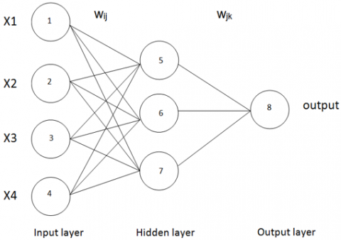
A neural network is a massively parallel distributed processor that has been developed for simple processing units, which has a natural propensity to store experiential knowledge and to make this knowledge available to be used. In two ways, the technique is analogous to the brain. The first similarity is that the network acquires knowledge from its surroundings through learning. The second resemblance is that synaptic weight, or the strength of interneuron connections, is employed to store acquired knowledge. A learning algorithm is a mechanism used to carry out the learning process. This method's goal is to change the network's synaptic weights in a systematic way to achieve the intended design objectives [17]. ANNs are of two kinds: Feedforward neural networks and feed backward neural networks [18]. The input variable for the task is received on most networks at the input layer. This includes all variables that could have an impact on the result. The output model is the output layer consisting of network predicted values. Between the input and output layers, one or more hidden layers could exist. The weights (Wij) and (Wjk) that can be modified during exercise connect each layer's neurons to the next layer of neurons [19]. Figure 1 shows a three-layer neural network with a weight connection through neuron layers, composed of four input layer neurons, three hidden layer neurons, and one output layer.
Figure 1. Structure of the ANN model
Statistical models have conveniently been utilized to forecast hydrologic data depending on time series methods. Furthermore, among statistical time series approaches for forecasting, Regression and Autoregressive Integrated Moving Average (ARIMA) has been a popular model. The properties of some types of hydrologic time series had periodically varying parameters. A linear stochastic model, generally referred to as the ARIMA model, can be used to model this type of data. These models' assumptions will prevent them from capturing non-stationary and non-linearity in hydrologic series. As such, decision-makers need to focus on models alternative to the ANN when non-stationary and non-linearity are the key parameters forecasting [15].
In the past few years, the ANN technique has been extensively utilized to model nonlinear and non-stationary time series in hydrology which has performed well in comparison to other statistical approaches. ANN is used in hydrologic and hydro-mechanical field modelling to estimate the values of variables such as river flow [20], sediment transport prediction [21, 22]. Some of these researches include flow rate estimation, rainfall, runoff modelling [23], and reservoir operation [24].
The back-propagation network is the most often used ANN model [25]. The back-propagation method specifies how to change the weight (Wij) and (Wjk) in any forward feed network to learn a training vector of input-output pairs. It is a supervised learning approach in which an output error is sent back into the network, changing connection weight to minimize the error between the network output and the goal output. As a result, back-propagation is employed as a method of ANN training in this case. The hidden layer's outputs are gathered and processed by the final or output layer, which provides the ultimate output.
To demonstrate the relevance and capabilities of the ANN for river level calculations, the Shaikh Hadeed station in western Iraq, downstream of the Haditha Dam, was selected as a case study region (see Figure 2). It is located at 41°55′–42°27′E and 34°13′–34°40′ N.
Figure 2. Location of Shaikh Hadeed station
At this station, river stage measurements are taken on a daily and monthly basis. Using the data sets stated, daily and monthly levels of the Euphrates were determined for the period (from 18/11/2007 to 27/03/2009) for the daily model and the period (from January 1986 to March 2009). This data was obtained from the Engineering Consulting Bureau at the University of Anbar [26]. The data set inspections show that water levels are highly dependent on the operational status of the Haditha Dam. In fact, during August (recession season), maximum water content was observed because of the massive amounts of water released for agricultural uses in this season (especially rice irrigation), while the lowest levels were observed around December. Because the area of catchment providing additional water to the Euphrates runs downstream of Haditha Dam, the levels of water, in addition to the state of operation of the dam, will also be affected by climatic conditions (the volume of precipitation).
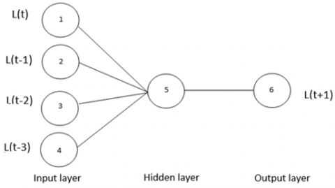
The methodology of this study is to use the available levels of observed data for the daily model (from 18/11/2007 to 27/03/2009) and the monthly model (January 1986 - March 2009). As a consequence, 496 and 241 instances of two models for predicting river level are presented, respectively. In MATLAB, a neural network with four nodes in the input layer and one node in the output layer is considered (see Figure 3). The transfer functions (tangent sigmoid – tangent sigmoid) were used in the daily model and (sigmoid – tangent sigmoid) in the monthly model; tangent sigmoid at the hidden layer and tangent sigmoid at the output in the daily model; and sigmoid at hidden layer and tangent sigmoid at the output in the monthly model. The input and target vectors were separated into three groups: (first set for training, the second set used to validate that the network is generalizing and stopping training before overfitting, and the third set used as a completely independent test of network generalization) [27].
In the two models, the default number of hidden neurons is (1,2, 3, 4, 5, ..., 9). Different nodes in the hidden layer are chosen to identify the optimal number of nodes in the hidden layer by trial and error. We conclude that the ideal number of nodes is one node in the hidden layer for the nine nodes listed previously. There are several algorithms available for training and changing the weight of a network. The Levenberg– Marquardt (trainLM) technique was used in this work since it is suggested for most issues [28].
Scaling the input and output variables before training is necessary to reduce their dimension and ensure that all variables are given equal attention during training. The input and output are normalized to have a zero mean and a unity standard deviation during the scaling process [25]. Depending on the output transfer function, the data is scaled using Eq. (1) below:
$X n=\frac{2(X-X \min )}{(X \max -X \min )}-1$ (1)
Figure 3. Structure of the ANN optimal model
The model's output depends on the types of transfer functions used in the hidden and output layers. Several transfer functions are used in ANN modelling, the most frequent of which are the liner, sigmoid, and tangent sigmoid. The following equations are the mathematical formulas for output equations created by a basic regression neural network that predicts new formations:
$I_{j}=\sum_{w_{i j} x_{i}}+\theta_{j}$ (2)
For tangent sigmoid function:
$f\left(I_{j}\right)=\frac{e^{\left(I_{j}\right)}-e^{-\left(I_{j}\right)}}{e^{\left(I_{j}\right)}+e^{-\left(I_{j}\right)}}$ (3)
For sigmoid function:
$f\left(I_{j}\right)=\frac{1}{1+e^{-\left(I_{j}\right)}}$ (4)
$I_{2 j}=\sum f\left(I_{j}\right) w_{j k}+\theta_{k}$ (5)
$O_{k}=\operatorname{TANH}\left(I_{2 j}\right)$ (6)
where, Ij = the activation level of node j, xi = the input from node i, i=1, 2, 3, 4, j=1, 2, 3, 4, …, 9 (hidden layer nodes), k=1 (output layer node), I2j = the activation level of node k, wij and wjk are training Weights given in Table 1, $\theta_{j}$= bias in a hidden layer, $\theta_{k}$ = bias in the output layer, Ok = Calculated outputs.
Table 1. Weights and threshold values for the ANN optimum model
(a) Daily model
|
Weight and Bias from the input layer(I) to the hidden layer(H) |
Weight and Bias from the hidden layer(H) to the output layer(O) |
||
|
H |
H |
||
|
I1 |
0.168680 |
O |
1.02600 |
|
I2 |
0.074852 |
||
|
I3 |
0.225110 |
||
|
I4 |
0.800660 |
||
|
Bias |
-0.518400 |
Bias |
0.45842 |
(b) Monthly model
|
Weight and Bias from the input layer(I) to the hidden layer(H) |
Weight and Bias from the hidden layer(H) to the output layer(O) |
||
|
H |
H |
||
|
I1 |
0.61802 |
O |
7.0213 |
|
I2 |
-0.093751 |
||
|
I3 |
0.047271 |
||
|
I4 |
0.0030298 |
||
|
Bias |
0.41672 |
Bias |
-4.2486 |
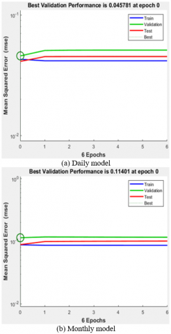
The model's training was terminated when the output was reasonable due to the following factors:
- The final mean-square error was small.
- The test set error and the validation set error are both comparable.
-There has been no evidence of considerable over fitting (where the best validation performance occurs) as seen in Figure 4.
Figure 4. Training, validation, and test errors
The data utilized to calibrate and validate the neural network models downstream of the Haditha Dam was obtained from the Shaikh Hadeed station. They were employed in the current study for model development and validation. ANN is used to identify the regression between observed and predicted output, dependent on the number of hidden layer nodes, mean square error, optimal validation performance, and transfer functions. The study concluded with two equations that can be used to predict daily and monthly water levels (t+1) with excellent regression.
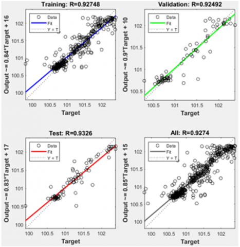
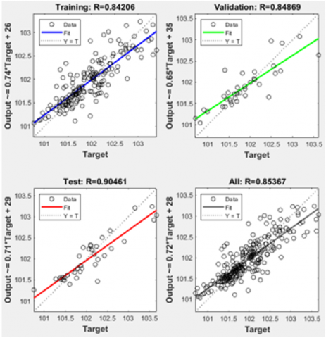
The regression was greater than 92 percent for all testing, validation, training, and all data for the daily model, and it was greater than 84 percent for the monthly model (see Figure 5).
Using the weights and bias indicated in Table 1(a) and the transfer function employed in the network, the daily anticipated water level [L(t+1)]d may be determined as follows:
$\operatorname{Level}(t+1) d=1.3 *(\tanh (1.026 * \tanh (x 1))+0.45842)+101.1$ (7)
where,
$\tanh (x 1)=\frac{e^{x 1}-e^{-x 1}}{e^{x 1}+e^{-x 1}}$
$x 1=\frac{L(t)}{1.6237}+\frac{L(t-1)}{5.77}+\frac{L(t-2)}{17.37}+\frac{L(t-3)}{7.71}-99.23$
(a) Daily model
(b) Monthly model
Figure 5. The regressions between observed (Target) - predicted (Output) L(t+1) for (Training, Validation, Test and All data)
The input units of Eq. (7) are the current and past days and have the following names:
L(t) = The present-day water level.
L(t-1) = Previous day water level.
L(t-2) = Two days ago water level.
L(t-3) = three days ago water level.
The equation's output is:
L(t+1)d = next day's water level.
The equation water level (t+1)d is only applicable to the level range (input value) between (99.8 - 102.4) m. This is because ANN should be used only for interpolation rather than extrapolation [18].
Figure 6. The input variables' relative relevance in the ANN daily model
As shown in Figure 6, the results show that the water level (t), water level (t-1), water level (t-2), and water level (t-3) all influenced the forecasted water level (t+1) with a relative importance of 63.08, 17.73, 5.89, and 13.28 percent, respectively. By converting the equation produced from the ANN model into a set of design diagrams, the veracity of the anticipated daily level of the river can be graphically verified..
On the other hand, using the weights and bias shown in Table 1 (b) and the transfer function applied in the network, the monthly forecast water level [L(t+1)]m can be calculated as follows:
$\operatorname{Level}(t+1) m=1.483333 *(\tanh (7.1444 *(\operatorname{Sig}(x l))-4.286))+102.1867$ (8)
where,
$\operatorname{Sig}(x 1)=\frac{1}{1+e^{-x 1}}$
$x 1=\frac{L(t)}{2.400}-\frac{L(t-1)}{15.822}+\frac{L(t-2)}{31.3794}+\frac{L(t-3)}{489.5813}-39.1653$
The inputs of Eq. (8) are as follows: The current month's average water level and previous months' averages were named as follows:
L(t) = The average of the current month's water level.
L(t-1) = The average of the previous month's water level.
L(t-2) = The average water level two months ago.
L(t-3) = The average water level three months ago.
The output of the equation is as follows:
L(t+1)m = The average of the next month's water level.
It is important to note that the equation (Level(t+1)m) is only valid for the range of levels between (100.70 - 103.67) m. As we have already stated, ANN should only be used for interpolation rather than extrapolation [18].
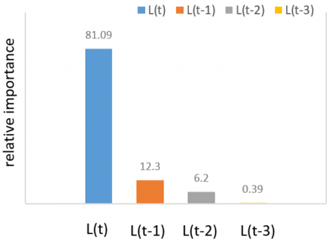
The findings indicated, that the predicted water level (t+1)m was 81.09, 12.3, 6.2 and 0.39 percent, respectively, as shown in Figure 7 and was water level (t-1), water level(t-2), water level ( t-3) with relative significance.
We may neglect the fourth input (water level (t-3)) depending on such results, due to its small water level impact (t+1)m. The credibility of the expected monthly river level can be graphically assessed by converting the equation from the ANN model into a design chart.
Figure 7. The input variables' relative relevance in the ANN monthly model
(a) Daily model
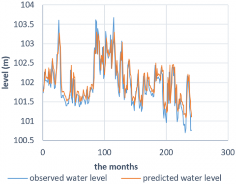
(b) Monthly model
Figure 8. The comparison between predicted values and observed
Figure 8 presents a comparison between the predicted and observed values in the daily and monthly models. As expected, he figure shows that the daily model is more accurate than the monthly model. The success of the ANN application depends on both the quality and the quantity of the input data. The optimal data set for training is that which is representative of the entire modeling domain [29, 30]. When the data for the daily model was compared with the data of the monthly model, the daily model accurately showed the process of change in levels more than the monthly model. This led to the quality of the data in the daily model being better than those for the monthly model. . Furthermore, the amount of data used for training in the daily model was greater than that utilized in the monthly model, which added a strength factor to the daily model.
The ANN approach was established in this work for determining the levels of the Euphrates River downstream of the Haditha dam using the backpropagation method. The following are the study's most significant findings:
- The Euphrates River application of ANN demonstrated that the ANN approach can be used to estimate river levels.
- The daily model is more accurate than the monthly model because the daily model training data is larger and the daily model water levels are more stable. Therefore, when the ANN model was well trained for regular events, it had better prediction quality.
- Month (t-3) has a negligible effect on month (t+1), due to the much greater time interval between the two periods.
[1] Almawla A.S., Kamel, A.H., Lateef, A.M. (2021). Modelling of flow patterns over spillway with CFD (Case study: Haditha Dam in Iraq. International Journal of Design & Nature and Ecodynamics, 16(4): 373-385. https://doi.org/10.18280/ijdne.160404
[2] Oyebode, O., Stretch, D.S. (2018). Neural network modelling of hydrological systems: A review of implementatio techniques. Natural Resource Modeling, 32(1): e12189. https://doi.org/10.1111/nrm.12189
[3] Karimi-Googhari, S., Feng, H.Y., Ghazali, A.H.B., Shui, L.T. (2010). Neural networks for forecasting daily reservoir inflows. Pertanika J. Sci. and Technol, 18(1): 33-41.
[4] Tanty, R., Desmukh, T.S. (2015). Application of artificial neural network in hydrology - A review. Int. J. Eng. Technol. Res, 4: 184-188. https://doi.org/10.17577/ijertv4is060247
[5] Nastos, P.T., Moustris, K. P., Larissi, I.K., Paliatsos, A.G. (2013). Rain intensity forecast using artificial neural networks in Athens, Greece. Atmospheric Research, 119: 153-160. https://doi.org/10.1016/j.atmosres.2011.07.020
[6] Nastos, P.T., Paliatsos, A.G., Koukouletsos, K.V., Larissi, I.K., Moustris, K.P. (2014). Artificial neural networks modeling for forecasting the maximum daily total precipitation at Athens, Greece. Atmospheric Research, 144: 141-150. https://doi.org/10.1016/j.atmosres.2013.11.013
[7] Nayak, D.R., Mahapatra, A., Mishra, P. (2013). A survey on rainfall prediction using artificial neural network. International Journal of Computer Applications, 72(16): 32-40. https://doi.org/10.5120/12580-9217
[8] MuttalebAlhashimi, S.A. (2014). Prediction of monthly rainfall in Kirkuk using artificial neural network and time series models. Journal of Engineering and Development, 18(1): 129-143.
[9] Neto, L.B., Coelho, P.H.G., Velloso, M.L.F., de Mello, J.C.C.B., Meza, L.A. (2004). Monthly flow estimation using elman neural networks. Proceedings of the Sixth International Conference on Enterprise Information Systems, pp. 153-158. https://doi.org/10.5220/0002610101530158
[10] Awchi, T.A. (2014). River discharges forecasting in northern Iraq using different ANN techniques. Water Resources Management, 28(3): 801-814. https://doi.org/10.1007/s11269-014-0516-3
[11] Zhou, J., Peng, T., Zhang, C., Sun, N. (2018). Data pre-analysis and ensemble of various artificial neural networks for monthly streamflow forecasting. Water, 10(5): 628. https://doi.org/10.3390/w10050628
[12] Chen, W.B., Liu, W.C. (2014). Artificial neural network modeling of dissolved oxygen in reservoir. Environmental Monitoring and Assessment, 186(2): 1203-1217. https://doi.org/10.1007/s10661-013-3450-6
[13] Ahmed, A.A.M. (2017). Prediction of dissolved oxygen in Surma River by biochemical oxygen demand and chemical oxygen demand using the artificial neural networks (ANNs). Journal of King Saud University - Engineering Sciences, 29(2): 151-158. https://doi.org/10.1016/j.jksues.2014.05.001
[14] Lohani, A.K., Kumar, R., Singh, R.D. (2012). Hydrological time series modeling: A comparison between adaptive neuro-fuzzy, neural network and autoregressive techniques. Journal of Hydrology, 442-443(6): 23-35. https://doi.org/10.1016/j.jhydrol.2012.03.031
[15] Sattari, M.T., Pal, K.Y.M. (2012). Performance evaluation of artificial neural network approaches in forecasting reservoir inflow. Applied Mathematical Modelling, 36(6): 2649-2657. https://doi.org/10.1016/j.apm.2011.09.048
[16] Yadav, A.K., Chandola, V.K., Singh, A., Singh, B.P. (2020). Rainfall-runoff modelling using artificial neural networks (ANNs) model. Int. J. Curr. Microbiol. App. Sci, 9(3): 127-135. https://doi.org/10.20546/ijcmas.2020.903.016
[17] Haykin, S. (1999). Neural Networks: A Comprehensive Foundation. Mac-Millan, New York.
[18] Abiodun, O.I., Jantan, A., Omolara, A.E., Dada, K.V., Mohamed, N.A., Arshad, H. (2018). State-of-the-art in artificial neural network applications: A survey. Heliyon, 4(11): e00938. https://doi.org/10.1016/j.heliyon.2018.e00938
[19] Al Aboodi, A.H., Dawood, A.S., Abbas, S.A. (2009). Prediction of tigris river stage in Qurna, South of Iraq, using artificial neural networks. Engineering and Technology Journal, 27(13): 2448-2450.
[20] Anika, N., Kato, T. (2019). Modeling river flow using artificial neural networks: A case study on Sumani watershed. Pertanika J. Sci. & Technol., 27(S1): 179-188.
[21] Rahman, S.A., Chakrabarty, D. (2020). Sediment transport modelling in an alluvial river with artificial neural network. Journal of Hydrology, 588: 125056. https://doi.org/10.1016/j.jhydrol.2020.125056
[22] Agarwal, A., Mishra, S.K., Ram, S., Singh, J.K. (2006). Simulation of runoff and sediment yield using artificial neural networks. Biosystems Engineering, 94(4): 597-613. https://doi.org/10.1016/j.biosystemseng.2006.02.014
[23] Atayi M.A. (2017). Rainfall-runoff modeling using artificial neural networks and HEC- HMS (Case study: Catchment of gharasoo), International Journal of Engineering Research, 6(7): 353-356. https://doi.org/10.5958/2319-6890.2017.00036.8
[24] Zhang, D., Peng, Q., Lin, J., Wang, D., Liu, X., Zhuang, J. (2019). Simulating reservoir operation using a recurrent neural network algorithm. Water, 11(4): 865. https://doi.org/10.3390/w11040865
[25] Mahmood, K.R., Aziz J. (2010). Using artificial neural networks for evaluation of collapse potential of some Iraqi Gypseous Soils. Iraqi Journal of Civil Engineering, 7( 1) : 21-28.
[26] Hydrological and Biological Study for the Euphrates at Al-Anbar Thermal Power Station, Engineering Consulting Bureau, University of Anbar. (2009). Unpublished Report.
[27] Shahin, M.A. (2003). Use of artificial neural networks for predicting settlement of shallow foundations on cohesionless soils. Ph.D. Thesis, Department of Civil and Environmental Eng., University of Adelaide .
[28] Almawla, A.S. (2017). Predicting the daily evaporation in ramadi city by using artificial neural network. Anbar Journal of Engineering Sciences, 7(2): 134-139.
[29] ASCE Task Committee on Application of Artificial Neural Networks in Hydrology. (2000). Artificial neural networks in hydrology. I: Preliminary concepts. Journal of Hydrologic Engineering, 5(2): 115-123. https://doi.org/10.1061/(ASCE)1084-0699(2000)5:2(115)
[30] ASCE Task Committee on Application of Artificial Neural Networks in Hydrology. (2000). Artificial neural networks in hydrology. II: Hydrologic applications. Journal of Hydrologic Engineering, 5(2): 124-137. https://doi.org/10.1061/(ASCE)1084-0699(2000)5:2(124)