Kamilia Sharir | Rodeano Roslee*
© 2022 IIETA. This article is published by IIETA and is licensed under the CC BY 4.0 license (http://creativecommons.org/licenses/by/4.0/).
OPEN ACCESS
The flood is one of the most devastating natural disasters to strike Sabah, Malaysia, especially in the Kota Belud region. The Flood Susceptibility Analysis (FSA) was described using bivariate statistical analysis (the Frequency Ratio model) based on a Geographical Information System (GIS). Field surveys and formal reports from local authorities in the study area created the flood inventory map. The training dataset for statistical analysis consisted of 100 flood locations inundated in 2017, while the validation dataset consisted of 54 flood locations from the 2016 flood report. Eight (8) parameters (elevation, slope curvature, slope angle, topography wetness index, drainage density, drainage proximity, land use, and soil type) were extracted from the database and then converted into a raster format with a cell size of 5m x 5m. Finally, using the natural break classification method, the FSA was generated and classified into five classes: very low, low, moderate, high, and very high susceptibility. The area under the curve (AUC) analysis validated the flood susceptibility model's accuracy. The success rate AUC was calculated to be 0.89, while the prediction rate AUC was 0.82. The flood susceptibility analysis could be used to develop flood mitigation strategies in land use planning.
flood susceptibility analysis, frequency ratio, Kota Belud, GIS, geospatial
Floods are the most common and destructive natural disasters that harm human health and natural environments [1, 2]. Flood hazard was becoming one of the dangerous natural hazards in Kota Belud, Sabah, Malaysia, resulting in extensive damage to properties infrastructures and impacting the local social economy. In 2017, this disaster affected approximately 4,441 people in 62 localities. The increase in the flood frequency and magnitude is related to heavy rains caused by monsoons or typhoons from neighboring countries, but it is also associated with the effects of the Ranau 2015 earthquake, with a magnitude of 6.0 on the Richter's scale. This situation causes the riverbed to become shallower due to it being filled with sediment deposits resulting from debris and woodpiles [3-11].
FSA mapping is an essential component of early warning systems or strategies for preventing and mitigating future flood situations, which aids in reducing the adverse effects of flood hazards. FSA mapping can be considered one of the risk assessment methods [12-14]. Risk is the product of susceptibility, hazard, and elements at risk, and it relates to the potential loss or damage produced by an event within that area. The susceptibility indicates the probability of a specific type occurring in each location, whereas the hazard refers to the likelihood of an event of a specific type and magnitude occurring in each location within a reference period [12]. This means that susceptibility can be used to predict the spatial occurrence of an event, whereas hazard can be used to predict the Spatio-temporal occurrence of an event. Even though the terms susceptibility and hazard have different meanings, they are always used interchangeably in geohazard research [15-19].
This study will use a statistical-bivariate Frequency Ratio model to produce a FSA map. This model was selected because the statistical-bivariate method has advantages over the statistical-multivariate method in terms of the techniques used for correlation analysis between the two variables [20-22]. This method combines the views of experts or the results of previous researchers in the selection of factors causing floods with the correlation of statistical techniques [16-19]. This method can study and evaluate flood hazards separately for each parameter used to map flood hazards. The integration of the statistical approach and the geographic information system aids in determining the value of the produced weights [1, 23, 24]. Hence, the primary goal of this research is to determine the Flood Susceptibility Level (FSL) using a GIS-based Frequency Ratio (FR) model.
The research was conducted in Kota Belud, Sabah, Malaysia, over a total area of 124km2. The study area's longitudinal and latitudinal extensions are 116°28'37.631"E–116°18'47.156"E and 6°18'32.655"N–6°25'49.605"N, respectively (Figure 1). This area's topography is dominated by a lowland in the northwestern corner and a hilly region in the south. As for the ground, the soils consist of clayey and loamy. The dominant bedrocks are sedimentary rocks, especially coastal and riverine alluvium. There are five main rivers, namely as Sungai Kadamaian, Sungai Wariu, Sungai, Gurong-Gurong, Sungai Tempasuk, and Sungai Abai, which always involved in a flood event.
The climate of the area belongs to tropical weather throughout the year with average daily temperature ranges from 21℃ to 32℃ [25]. The climate of Kota Belud is typically influenced by winds from the Indian Ocean (Southwest Monsoon - May to September) and the South China Sea (North-Eastern Monsoon - November to March). The annual precipitation average is 492.4 mm [25]. All activities, such as mapping, assessment, and investigating, are concentrated in the lowland area, which is prone to flooding.
It is critical to examine the occurrence of previous flood events in order to forecast future floods in the study area. The study utilized a geospatial-based methodology for FSA mapping. The GIS-based FR method has been used to analyse the flood-prone area. The methods used in this study aim to conduct the FSA consisting of three stages; (stage 1) flood inventory – which is the process to identify and characterize the flood event from a field survey along with handheld GPS, (stage 2) flood causative conditioning factors – their area eight parameters were used as the causative factors to flooding (elevation, slope curvature, slope angle, topography wetness index, drainage density, drainage proximity, land use, and soil type) and (stage 3) Frequency Ratio (FR) model - the FSA was defined using a Geographical Information System (GIS) based-bivariate statistical analysis, and then validate the model using the area Under the Curve (AUC).
3.1 Flood Hazard Inventory (FHI)
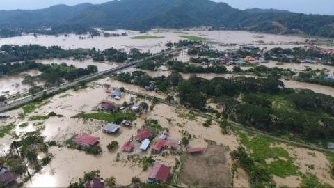
The delineating flooded area is the most critical component whenever dealing with flood susceptibility mapping. Initial identification of flooded area locations from the field survey and published reports from government agencies may be used to obtain significantly. The field observations were carried out during and after the 2017 flood events to collect accurate data for FSA mapping (Figure 1).
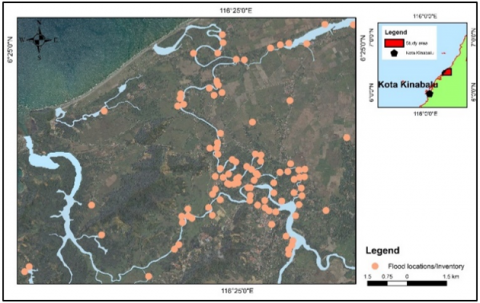
A total of 100 flood locations were identified and located on the map. The training dataset for the model was the total number of flood locations from the 2017 field survey, and previous flood data from 2016 (54 flood locations) was used to validate the FSA model (Figure 2).
Figure 1. Field investigation during and after the flood events of 2017
Figure 2. Flood inventory map in the study area
3.2 Flood causative factors
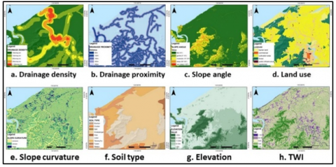
The study utilized a geospatial-based methodology for flood susceptibility mapping. Selection of the valuable parameter for the flood hazard map in any area is essential, and it is challenging to choose factors commonly used in flood susceptibility mapping [26]. ArcGIS software prepared the eight physical factors contributing to flood occurrences, such as elevation, slope curvature, slope angle, topography wetness index, drainage density, drainage proximity, land use, and soil type. All of the causative factors in the FR model were adopted after doing a literature review and conducting a reconnaissance survey to understand the flood conditions that frequently cause floods in the study area. (Figure 3). The more reliable the conditioning parameters, the more accurate the flood susceptibility zonation will be.
Digital Elevation Model (DEM) is the primary source to build the model because it contains information about topographic attributes that can help flood analysis [27]. Interferometric Synthetic-Aperture Radar (IFSAR) data with the 5m spatial resolution are used and processed for the DEM. Timbalai RSO Borneo (meters) was used to rectify the dataset. This study used DEM to extract elevation, slope angle, slope curvature, and topographic wetness index.
Figure 3. Flood causative factors used in FR model
In the analysis of assessing and mapping flood susceptibility, one of the crucial parameters in flood control is topographic elevation [28]. The elevation was classified to 5 classes; <5m, 6-10m, 11-20m, 21-30m and >30m. The Topographic Wetness Index (TWI) shows the total accumulation of water flow at any point in the drainage basin and the ability of water to flow down by gravity [26]. TWI has a significant effect on flood mapping [29]. The TWI has no unit and was classified into five classes: <5, 5-6, 6-8, 8-10, >10 using the natural break jenk method.
Slope curvature is classified into three types: convex, concave, and horizontal. Slope curvature also influences infiltration and the rate of surface water runoff. Positive curvature represents that the slope gradient is convex in an upward direction, whereas negative curvature indicates that the slope gradient is concave upwardly, and the slope gradient will be flat if the value is zero [30].
In addition to topographic altitude, one of the essential topographic factors in hydrological studies is slope angle, which is essential in controlling the flow of water at the water's surface. The slope angle controls the surface runoff [29]. Low gradient slopes are more prone to flooding than high gradient slopes [31]. The slope angle was classified into five classes based on the slope classification published by the Department of Mineral and Geoscience Malaysia (JMG, 2006); flat (<5°), gentle (5°-15°), moderate (15°-25°), steep (25°-35°) and very steep (>35°).
Land use directly or indirectly affects the rate of infiltration, evapotranspiration, and generation of surface water runoff [29]. The land use map was prepared from the topography map and was classified into six classes: barren land, commercial, cultivation area, forest, public infrastructure, and residential area. Infiltration is affected by the spatial variability of soil type and regulates overland flows and flooding [29]. Therefore, soil type was prepared based on soil data derived from the Agriculture Department of Sabah (JPNS, 1976).
In general, flood events usually occur around drainage systems. Therefore, taking into account the buffer zone (distance) to drainage is an important parameter to ensure the accuracy of flood hazard maps (Sumit Das, 2018). Furthermore, the lowest point in an area is often closely related to the presence of a drainage system [29]. The higher the drainage density, the larger the catchment area susceptible to erosion, resulting in sedimentation at the lower ground [31]. The drainage density was calculated by dividing the total length of the drainage channel in the watershed by the watershed's total area. The topography map of the study area could be used to derive data, drainage density, and a proximity map.
3.3 Frequency Ratio (FR)
The FR model can be used to quickly assess geospatially the probabilistic relationship of databases with various levels of classification between dependent or independent variables [32]. For the calculation of the FR, the ratio of the range of flood occurrence zone and the flood-unaffected area is determined for each class or type of factor, and the ratio of this area is calculated in each factor category to the overall range. The description of this definition is explained simply using the following equation as Eq. (1):
$F R=\frac{\text { Percentage flood area }(\%)}{\text { Percentage pixels number in domain }(\%)}$ (1)
The FR model is used to predict the association between previous flood events and the variables (or parameters) that influence those events [33]. If the result of the FR value obtained is below the value of 1 (one), then this value indicates that the correlation between flood events and the variable is weak. If the opposite happens, the FR value exceeds the value of 1 (one), then this value indicates the strong correlation between the variable and the occurrence of flooding. These calculations were made using the training data set as well as the validation data set to obtain the accuracy of the model generated through this method. Both of these data sets will go through the same steps in generating this model. To construct a flood susceptibility map using this method, the values obtained through the calculation of the FR for each factor (variable) will be summed in a "raster calculator" using ArcGIS software to obtain the final result, as shown in the equation Eq. (2). The produced map was classified into 5 zones ranging from very low to very high susceptibility zones using natural break method.
F S M=$\Sigma$ frequency ratio in each factor type (2)
By comparing it to the flood inventory map, the FSM produced by the FR model for the study area was validated. In this study, the success rate curve was calculated to assess the efficacy of the FR model and factors used to predict floods. To generate the success rate curve, the relative ranks for each prediction pattern were calculated and sorted in descending order by calculating the index values of all cells in the study area. To calculate the percentage of floods in each susceptible class, the 100 classes were overlaid and intersected with the training dataset used to generate the model. The success rate curve was then constructed by plotting the susceptible classes from highest to lowest values on the X-axis and the cumulative percentage of flood occurrences on the Y-axis.
By calculating the prediction rate, the susceptibility map was also evaluated in terms of predictive power and validity. To create the prediction rate curve, the flood validation dataset was used instead of the flood training dataset, which was created using the same data integration and representation processes described above. If the slope of the curve graph is steeper, it indicates that there are more floods in the highly susceptibility category. The AUC range is varied, from 0.6 to 1.0. The highest accuracy has a value of 1.0, thus indicating that the model's performance is very satisfactory in predicting the occurrence of disasters without any tendency. Therefore, AUC values closer to 1.0 indicate that the model has high accuracy and reliability.
The FSA mapping in the study area has been analysed with its eight causative factors and correlate them with flood inventory using FR method. Each factor was classified as weight by the FR values shown in Table 1.
The drainage proximity ranges between 100m, 150m, and 200m showed the highest values of FR; 2.33, 2.05, and 1.28, respectively. This analysis indicates that the flood takes place to close the riverbank and is very uncommonly far from the river. The relationship between flood inventory and drainage density shows that areas of 20km/ sq km, 25km/ sq km, and >30km/ sq km are more likely to flood, with a ratio of 2.00, 5.47, and 6.21, respectively.
For the slope curvature, linear (or flat) areas proved to be the most prone to flooding, with the highest FR value of 2.00. In comparison, the relationship between flood inventory and slope angle exposes that <5⁰ have the highest possibility of flood occurrence with an FR value of 2.00, and the FR value decreases as the slope angle increase, which means that chances of flood decrease with an increase in slope angle.
Table 1. The FR analysis in each factor class
|
Factor |
Class |
% pixels no. in domain |
% flood location |
FR |
|
|
10km/ km2 |
54.71 |
6 |
0.11 |
|
|
15km/ km2 |
25.33 |
21 |
0.83 |
|
1.DD |
20km/ km2 |
10.99 |
22 |
2.00 |
|
|
25km/ km2 |
6.40 |
35 |
5.47 |
|
|
> 30km/ km2 |
2.58 |
16 |
6.21 |
|
|
|
|
|
|
|
|
50m |
19.18 |
7 |
0.37 |
|
|
100m |
16.72 |
39 |
2.33 |
|
2.DP |
150m |
12.71 |
26 |
2.05 |
|
|
200m |
9.34 |
12 |
1.28 |
|
|
250m |
42.06 |
16 |
0.38 |
|
|
|
|
|
|
|
|
Convex |
51.01 |
50 |
0.98 |
|
3.SC |
Linear |
6.49 |
13 |
2.00 |
|
|
Concave |
42.49 |
37 |
0.87 |
|
|
|
|
|
|
|
|
Cultivation area |
43.61 |
36 |
0.83 |
|
|
Commercial |
0.36 |
0 |
0.00 |
|
4.LU |
Barren land |
4.75 |
7 |
1.48 |
|
|
Forest |
38.01 |
4 |
0.11 |
|
|
Public infrastructure |
0.61 |
2 |
3.28 |
|
|
Residential |
12.67 |
51 |
4.03 |
|
|
|
|
|
|
|
|
<5m |
42.42 |
29 |
0.68 |
|
|
6 - 10m |
22.64 |
62 |
2.74 |
|
5.EL |
11 - 20m |
13.15 |
9 |
0.68 |
|
|
20 - 30m |
4.43 |
0 |
0.00 |
|
|
>30m |
17.36 |
0 |
0.00 |
|
|
|
|
|
|
|
|
<5° |
71.67 |
98 |
1.37 |
|
|
5° - 15° |
13.52 |
2 |
0.15 |
|
6.SA |
15° - 25° |
11.30 |
0 |
0.00 |
|
|
25° - 35° |
3.39 |
0 |
0.00 |
|
|
>35° |
0.13 |
0 |
0.00 |
|
|
|
|
|
|
|
|
Weston |
13.21 |
1 |
0.08 |
|
|
Brantian |
0.05 |
0 |
0.00 |
|
|
Tanjong Aru |
11.47 |
2 |
0.17 |
|
|
Dalit |
0.03 |
0 |
0.00 |
|
7.ST |
Lokan |
31.38 |
11 |
0.35 |
|
|
Tuaran |
0.61 |
0 |
0.00 |
|
|
Crocker |
0.04 |
0 |
0.00 |
|
|
Kinabatangan |
42.85 |
86 |
2.01 |
|
|
Klias |
0.36 |
0 |
0.00 |
|
|
|
|
|
|
|
|
1-5 |
15.05 |
0 |
0.00 |
|
|
5-6 |
32.43 |
21 |
0.65 |
|
8.TWI |
6-8 |
31.79 |
49 |
1.54 |
|
|
8-10 |
16.37 |
23 |
1.40 |
|
|
>10 |
4.36 |
7 |
1.61 |
Notes: 1. DD=Drainage Density. 2. DP=Drainage Proximity. 3. SC=Slope Curvature. 4. Lu=Land Use. 5. EL= Elevation. 6. SA=Slope angle. 7. ST=Soil Type. 8. TWI=The Wetness Index.
Among land use classes, the highest FR was observed for the barren land, public infrastructure, and residential, with FR values of 1.48, 3.28, and 4.03, respectively. Results found that Kinabatangan has the highest FR values (2.01) for soil type. The landform usually associated with this soil type is flood plain, and the parent material for this soil type is alluvium. It is undeniable that this soil type is very prone to flood threats.
Besides, the FR model application found that most flooding hazards are located at elevations of 6-10m. Elevation class 6-10m has the highest FR value of 2.74. Elevations higher than this class had the lowest FR, and earlier work showed that in high elevation regions, flooding is unlikely to happen [29]. The FR values for the topographic wetness index (TWI) classes showed a general trend that increased with higher TWI values in the range of 6-8, 8-10, and >10, with 1.54, 1.40, and 1.61, respectively.
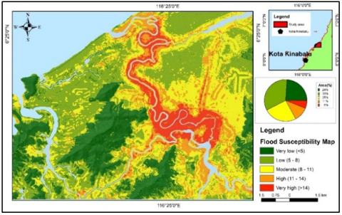
The rating layers for the various flood-related factors were built using the FR values. Figure 4 depicts the flood susceptibility map generated by the FR model. In the study area, the resulting flood susceptibility index values ranged from 1.54 to 22.3. The study area has been classified into five (5) flood susceptibility zones based on the natural break (jenk) classifier method: very low (<5), low (5 – 8), moderate (8 – 11), high (11 – 14), and very high (>14). (Table 2).
The flood susceptibility value represents the likelihood of flooding occurrence. As a result, the higher the FR values, the greater the susceptibility to flooding. According to the findings, 24% (47km2) of the area has very low susceptibility, 33% (65km2) has low susceptibility, 25% (49km2) has moderate susceptibility, and 11% (21km2) has high susceptibility, and 6% (12km2) has very high susceptibility. According to the findings, the very high susceptibility to flooding zones was mainly found along the major rivers in the study area, Sungai Tempasuk, Sungai Gurung-Gurung, and around the district center Pekan Kota Belud. The critical factors in the very high susceptibility flood zones were higher drainage density, proximity to the river, low slope angle, and elevation.
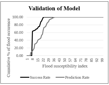
The model's validation should be examined to demonstrate how well the model was carried out [34]. The flood susceptibility map was validated by comparing it to flood inventory data. As shown in Figure 5, the cumulative percentage of flood occurrence was calculated, and the success rate curve was plotted. The success rate for final flood susceptibility validated using the area under the curve was 0.89 (89.13%), and the prediction rate was 0.82 (82.18%). The success rate curve was depicted in black, while a grey line represented the prediction rate. The highest accuracy (1.0) value indicated that the model was completely capable of predicting an event without bias [35, 36]. We can conclude from the validation values that this model is precise and trustworthy.
Figure 4. Flood susceptibility map (FSA)
Table 2. Spatial distribution of FSM classes in the study area
|
FSM class |
FR value range |
% area |
|
Very Low |
< 5.0 |
24% (47km2) |
|
Low |
5.0 – 8.0 |
33% (65km2) |
|
Moderate |
8.0 – 11.0 |
25% (49km2) |
|
High |
11.0 – 14.0 |
11% (21km2) |
|
Very High |
> 14.0 |
6% (12km2) |
Figure 5. Validation of flood susceptibility
This study shows that combining statistical bivariate FR and GIS technology provides a valuable decision-making tool for FSA mapping by allowing for consistent and effective use of spatial information. The training dataset consisted of 100 flood locations inundated in 2017, while the validation dataset consisted of 54 flood locations from the 2016 flood report. Eight conditioning parameters were used as independent variables (elevation, slope curvature, slope angle, topography wetness index, drainage density, drainage proximity, land use, and soil type).
Lastly, a FSA map was generated and classified into five classes (low, low, moderate, high, and very high). All layers used in this study were resampled into 5x5 meter spatial resolution to standardize the final map. The FSA map shows that the very high flood susceptibility area was located in the main river channel and around the district center. The AUC curve showed that this model is trustable, with a success and prediction rate of 0.89 and 0.82, respectively. The small number of flood locations used for modeling training and validation was one of the study's limitations. However, depending on the data availability, the method used in this study can be easily applied in other fields where different factors can be considered. As a result, this FR model has been successfully tested and is appropriate for selecting land-use suitability, controlling, and managing flood hazard/risk in the study area.
Sincere thanks to the Natural Disaster Research Centre (NDRC) and the Faculty of Science and Natural Resources (FSSA) at Universiti Malaysia Sabah (UMS) for making laboratories and research equipment available. Thank you also to the research grant award (SDK0012-2017) for covering all of the costs of this research.
[1] Samanta, R.K., Bhunia, G.S., Shit, P.K., Pourghasemi, H.R. (2018). Flood susceptibility mapping using geospatial frequency ratio technique: A case study of Subarnarekha River Basin, India. Model Earth Syst Environ., 4: 395-408. https://doi.org/10.1007/s40808-018-0427-z
[2] Zou, Q., Zhou, J., Zhou, C., Song, L., Guo, J. (2013). Comprehensive flood risk assessment based on set pair analysis-variable fuzzy sets model and fuzzy AHP. Stoch Environ Res Risk Assess., 27: 525-546. https://doi.org/10.1007/s00477-012-0598-5
[3] Ayog, J.L., Tongkul, F., Mirasa, A.K., Roslee, R., Dullah, S. (2017). Flood risk assessment on selected critical infrastructure in Kota Marudu Town, Sabah, Malaysia. MATEC Web of Conferences, 103: 04019(1)-04019(9). https://doi.org/10.1051/matecconf/201710304019
[4] Roslee, R., Jamaludin, T.A., Simon, N. (2017). Landslide Vulnerability Assessment (LVAs): A case study from Kota Kinabalu, Sabah, Malaysia. Indonesian Journal on Geoscience, 4 (1): 49-59. https://doi.org/10.17014/ijog.4.1.49-59
[5] Nicole L.S.L, Bolong, N., Roslee, R., Tongkul, F., Mirasa, A.K., Ayog, J.L. (2018). Flood vulnerability index for critical infrastructure towards flood risk management. ASM Sci. J., 11(3): 134-146.
[6] Roslee, R., Tongkul, F., Mariappan, S., Simon, N. (2018). Flood Hazard Analysis (FHAn) using multi-criteria evaluation (MCE) in Penampang Area, Sabah, Malaysia. ASM Sci. J., 11(3): 104-122.
[7] Roslee, R., Norhisham, M.N. (2018). Flood susceptibility analysis using multi-criteria evaluation model: A case study in Kota Kinabalu, Sabah. ASM Sci. J., 11(3): 123-133.
[8] Mariappan, S., Roslee, R., Sharir, K. (2019). Flood Susceptibility Analysis (FSAn) using Multi-Criteria Evaluation (MCE) technique for landuse planning: A case from Penampang, Sabah, Malaysia. Journal of Physics: Conference Series, 1358(2019): 012067. https://doi.org/10.1088/1742-6596/1358/1/012067
[9] Roslee, R., Sharir, K. (2019). Integration of GIS-based RUSLE model for land planning and environmental management in Ranau Area, Sabah, Malaysia. ASM Sc. J., 12(3): 60-69.
[10] Roslee, R., Sharir, K. (2019). Soil erosion analysis using RUSLE model at the Minitod area, Penampang, Sabah, Malaysia. Journal of Physics: Conference Series, 1358: 012066.
[11] Sharir, K., Roslee, R., Mariappan, S. (2019). Flood Susceptibility Analysis (FSA) using analytical hierarchy process (AHP) model at the Kg. Kolopis area, Penampang, Sabah, Malaysia. Journal of Physics: Conference Series, 1358: 012065. https://doi.org/10.1088/1742-6596/1358/1/012065
[12] Azemeraw, W., Gashaw, T., Zerihun, D., Belete, G., Tamirat M., Muralitharan, J. (2020). Comparison of statistical and analytical hierarchy process methods on flood susceptibility mapping: in a case study of Tana sub-basin in northwestern Ethiopia. Natural Hazards and Earth System Sciences, 1-43. https://doi.org/10.5194/nhess-2020-332
[13] Adger, N.W. (2006). Vulnerability, Glob. Environ. Chang., 16: 268-281. https://doi.org/10.1016/j.gloenvcha.2006.02.006
[14] Jacinto, R., Grosso, N., Reis, E., Dias, L., Santos, F.D., Garrett, P. (2015). Continental Portuguese Territory Flood Susceptibility Index—Contribution to a vulnerability index. Nat. Hazards Earth Syst. Sci., 15: 1907-1919. https://doi.org/10.5194/nhess-15-1907-2015
[15] Roslee, R., Bidin, K., Musta, B., Tahir, S. (2017). Intergration of GIS in estimation of soil erosion rate at Kota Kinabalu area, Sabah, Malaysia. Adv. Sci. Lett., 23(2): 1352-1356. https://doi.org/10.1166/asl.2017.8400
[16] Tehrany, M.S., Pradhan, B., Jebur, M.N. (2013). Spatial prediction of flood susceptible areas using rule based decision tree (DT) and a novel ensemble bivariate and multivariate statistical models in GIS. J Hydrol., 504: 69-79. https://doi.org/10.1016/j.jhydrol.2013.09.034
[17] Rahmati, O., Pourghasemi, H.R., Zeinivand, H. (2016). Flood susceptibility mapping using frequency ratio and weights-of-evidence models in the Golastan Province, Iran. Geocarto Int., 31: 42-70. https://doi.org/10.1080/10106049.2015.1041559
[18] Ozdemir, A., Altural, T. (2013). A comparative study of frequency ratio, weights of evidence and logistic regression methods for landslide susceptibility mapping: Sultan mountains, SW Turkey. J Asian Earth Sci., 64: 180-197. https://doi.org/10.1016/j.jseaes.2012.12.014
[19] Youssef, A.M., Pradhan, B., Sefry, S.A. (2016). Flash flood susceptibility assessment in Jeddah city (Kingdom of Saudi Arabia) using bivariate and multivariate statistical models. Environ Earth Sci., 75: 1-16. https://doi.org/10.1007/s12665-015-4830-8
[20] Aditian, A., Kubota, T., Shinohara, Y. (2018). Comparison of GIS-based landslide susceptibility models using frequency ratio, logistic regression, and artificial neural network in a tertiary region of Ambon, Indonesia. Geomorphology, 318: 101-111. https://doi.org/10.1016/j.geomorph.2018.06.006
[21] Shahabi, H., Ahmad, B.B., Khezri, S. (2013). Evaluation and comparison of bivariate and multivariate statistical methods for landslide susceptibility mapping (case study: Zab basin). Arab J Geosci., 6: 3885-3907. https://doi.org/10.1007/s12517-012-0650-2
[22] Shafapour, M., Jebur, M.N., Honghttps, H., Chen, W. (2017). GIS-based spatial prediction of flood prone areas using standalone frequency ratio, logistic regression, weight of evidence and their ensemble techniques. Geomatics, Natural Hazards and Risk, 8(2): 1538-1561. http://dx.doi.org/10.1080/19475705.2017.1362038
[23] Khosravi, K., Nohani, E., Maroufinia, E., Pourghasemi, H.R. (2016). A GIS-based flood susceptibility assessment and its mapping in Iran: A comparison between frequency ratio and weights-of-evidence bivariate statistical models with multi-criteria decision-making technique. Nat Hazards., 83: 947-987. https://doi.org/10.1007/s11069-016-2357-2
[24] Paul, G.C., Saha, S., Hembram, T.K. (2019). Application of the GIS-Based probabilistic models for mapping the flood susceptibility in Bansloi Sub-basin of Ganga-Bhagirathi River and Their Comparison. Remote Sens Earth Syst Sci., 2: 120-146. https://doi.org/10.1007/s41976-019-00018-6
[25] Jabatan Meteorologi Malaysia. (2021). Ramalan Cuaca Daerah Kota Belud. https://www.met.gov.my/forecast/weather/district/Ds558#.
[26] Tehrany, M.S., Pradhan, B., Jebur, M. (2014). Flood susceptibility mapping using a novel ensemble weights-of-evidence and support vector machine models in GIS. Journal Hydrology, 512: 332-343. https://doi.org/10.1016/j.jhydrol.2014.03.008
[27] Ul Moazzam, M.F., Vansarochana, C., Rahman, A.U. (2018). Analysis of flood susceptibility and zonation for risk management using frequency ratio model in District Charsadda, Pakistan. International Journal of Environment and Geoinformatics, 5(2): 140-153. https://doi.org/10.30897/ijegeo.407260
[28] Botzen, W.J.W., Aerts, J.C.J.H., van den Bergh, J.C.J.M. (2013). Individual preferences for reducing flood risk to near zero through elevation. Mitig. Adapt. Strateg. Glob. Chang., 18: 229-244. https://doi.org/10.1007/s11027-012-9359-5
[29] Samanta, S., Pal, D.K., Palsamanta, B. (2018). Flood susceptibility analysis through remote sensing, GIS and frequency ratio model. Applied Water Science, 8: 66. https://doi.org/10.1007/s13201-018-0710-1
[30] Ayalew, L., Yamagishi, H. (2005). The application of GIS-based logisti regression for landslide susceptibility mapping in the Kakuda-Yahiko Mountains, Central Japan. Geomorphology, 65(1-2): 15-31. https://doi.org/10.1016/j.geomorph.2004.06.010
[31] Ouma, Y.O., Tateishi, R. (2014). Urban flood vulnerability and risk mapping using integrated multi-parametric AHP and GIS: Methodological overview and case study assessment. Water, 6(6): 1515-1545. https://doi.org/10.3390/w6061515
[32] Laxton, J.L. (1996). Geographic information systems for geoscientists. Modelling with GIS, 10: 355-356.
[33] Intarawichian, N., Dasananda, S. (2011). Frequency ratio model based landslide susceptibility mapping in lower Mae Chaem watershed, Northern Thailand. Environmental Earth Sciences, 64(8): 2271-2285. https://doi.org/10.1007/s12665-011-1055-3
[34] Chung, C.J.F., Fabbri, A.G. (2003). Validation of spatial prediction models for landslide hazard mapping. Natural Hazards, 30(3): 451-472. https://doi.org/10.1023/B:NHAZ.0000007172.62651.2b
[35] Pradhan, B., Oh, H.J., Buchroithner, M. (2010). Weights-of-evidence model applied to landslide susceptibility mapping in a tropical hilly area. Geomat Nat Hazards Risk, 1: 199-223. https://doi.org/10.1080/19475705.2010.498151
[36] Kia, M.B., Pirasteh, S., Pradhan, B., Rodzi, M.A., Sulaiman, W.N.A., Moradi, A. (2012). An artificial neural network model for flood simulation using GIS: Johor River Basin, Malaysia. Environment Earth Science, 67: 251-264. https://doi.org/10.1007/s12665-011-1504-z