Ahmed Saud Mohammed* | Md Azlin Md Said | Ammar Hatem Kamel | Rozi Abdullah
© 2022 IIETA. This article is published by IIETA and is licensed under the CC BY 4.0 license (http://creativecommons.org/licenses/by/4.0/).
OPEN ACCESS
Evaporation is influenced by several meteorological parameters, evaporation data are usually difficult to obtain compared to rainfall data, especially in arid regions. Developing a monthly evaporation prediction model in arid regions in terms of available meteorological data is a significant step. The data used in this study for modeling are monthly measurements to cover substantial continuity over a period of 18 years between January 2000 and December 2017. Stepwise and backward multiple linear regression techniques were used with a new procedure of variable selection to select the best model. Temperature, wind speed, relative humidity and sunshine hours were used as a independent variables in the multiple linear regression (MLR) technique to establish the best prediction of the evaporation model. To examine the MLR evaporation developed model in the current study, MLR results were compared with the most common evaporation models commonly used in arid regions such as Kharufa and Khosla methods. The results of performance indicators shows that the R2 values are approximately 0.937, 0.90 and 0.85 for MLR evaporation developed model, Kharufa and Khosla methods, respectively. Moreover, the values of the error measures, namely RMSE and NAE for MLR evaporation developed model were 36.3 and 0.123, Kharufa model 71.22 and 0.241 and Khosla model was and 173.7 and 0.581 respectively. Based on the foregoing, the results of the MLR developed evaporation model in the current study outperforms in all performance indicators and proves to be better than the Kharufa and Khosla models.
evaporation, MLR, Horan valley, Kharufa, Khosla
Evaporation is a main element of the hydrologic cycle, it is considered a key factor in the management of water resources for arid and semi-arid regions. Estimating water loss through evaporation is essential for modeling, surveying and managing many hydrological and water resource systems projects [1-8]. In general, evaporation data is significantly less easily obtainable than rainfall data.
Evaporation is a variable that combines or incorporates the effects of many elements of the atmosphere, such as temperature, humidity, rainfall, solar radiation and wind speed [9, 10]. The evaporation increases with high wind speed, max temperatures and low humidity [7].
Potential evaporation is the potential or ability of the atmosphere to remove water from a surface if there is no limit to the water availability [11, 12]. Potential evaporation is the most commonly used variable, while actual evaporation is the amount of water removed by evaporation from that surface [13, 14].
Evaporation estimates are required for a variety of problems in water resource management, hydrology, river flow forecasting, land resources planning, agricultural, forestry, irrigation management, and ecosystem modeling.
Reservoir locations will be limited in arid areas with flat terrains, and reservoirs will likely be shallow and have large surface areas. In such cases evaporation can cause large amounts of water to be lost [15, 16]. As a result, estimating the evaporation losses will be crucial in evaluating the design and operation of these reservoirs. The measurement of evaporation in the open environment is difficult and is usually done by proxy and models can be useful for evaporation prediction methods.
The application of the multiple linear regression (MLR) technique for evaporation studies helps to penetrate the hidden interrelationships among different parameters in catchments arid regions and developed model to best predict the processes of evaporation [17]. The models developed from meteorological data involve empirical relationships to some extent, these models may give reliable results when applied to climatic conditions [14]. The use of formulas or mathematical models that can predict evaporation from available climate data is therefore assertive and can provide more precise results than the calculated evaporation [18-21]. These models had been widely used by several researchers to estimate evaporation based on meteorological parameters like [1, 9, 13, 19, 20, 22-25].
Cahoon et al. [26] and Fennessey and Vogel 1996 [27] used regression methods to create models for regional monthly average evaporation in the United States as a function of publicly available factors including temperature, longitude, and elevation. Hanson [28] investigated the daily evaporation on three sites on the watershed in southwest Idaho India. The study pointed to daily pan evaporation estimated by mean temperature and solar radiation, the correlation coefficients (r) were obtained between 0.84 to 0.90. Almedeij [25] investigated the evaporation in Kuwait state and reported that the correlation of evaporation with temperature was 0.94, RH was -0.92 and wind speed was 0.74. Almedeij [1] develop an evaporation model arid region using a monthly period of 23 years (1993-2015). The study showed that evaporation values, ranged between 0.1 to 40 mm/day, from January – July within this period.
The significance of this study emerged through the fact that accurately measuring evaporation is a difficult task, especially in arid regions. As a result, using equations or statistical models to predict pan evaporation from available meteorological data may provide more accurate results. The main aim of this study was to develop a monthly predict evaporation model using multiple linear regression that can be used to estimate monthly evaporation in arid regions and identify the internal relationships between the independent variables that contribute to the prediction of evaporation.
Horan valley, the largest valley in Iraq, is located in Al-Anbar governorate in western Iraq (see Figure 1), extending for a distance of 485 km from the Iraqi-Saudi border to the Euphrates River near Haditha region between the longitudes of (39 00' 00') and (43 00' 00") east and latitude (32 00' 00") and (43 30' 00") North. The valley catchment area is around 16550 km2 and the difference in elevation between upstream and downstream is around 600 m. Horan valley region is classified as an arid region characterized by hot summer and cold winter.
Figure 1. Horan valley location
Monthly climate data such as temperature (T), evaporation (E), relative humidity (RH), wind speed (WS) and solar brightness (SS) for the period 2000-2017 are provided from Iraqi Meteorological Organization Seismology (IMOS) in Baghdad presents six weather stations namely Ramadi, Haditha, Anah, Qaim, Rutba and Nakheb (see Figure 2).
Figure 2. Locations of the climatic station around the study area
Linear regression is one of the best used methods for linear modelling that is commonly used to analyze the relationship between a dependent (response) and several independents (predictors) variables. MLR can be expressed according to the following equation.
$y=b_{0}+b_{i} x_{i}+\cdots+b_{k} x_{k}+\varepsilon, i=1,2, \ldots k$ (1)
The linear regression method seeks to model the relationship between two variables based on the observed data for these two variables to produce the best suitable linear equation. The simplest models that can predict evaporation from its independent variables are statistical regression methods. These whole empirical techniques are quick and easy to apply since they do not require complex parameter input. A large number of models in hydrology and climate sciences have to depend on the multiple linear regression to justify the link between key variables.
Prediction accuracy analysis typically requires the estimation of errors between observed and predicted values. Five performance indicators were used in the current study such as root mean square error (RMSE), normalized absolute error (NAE), coefficient of determination (R2), Nash-Sutcliffe efficiency (NSE) and mean average percentage error (MAPE). NAE and RMSE should reach zero for a successful pattern, while NSE and R2 should be closer to one [7].
$\mathrm{R}^{2}=\left(\frac{\sum_{i-1}^{N}\left(P_{i}-\bar{P}\right)\left(O_{i}-\bar{O}\right)}{N . S_{\text {pred }} \cdot S_{o b s}}\right)^{2}$ (2)
$R M S E=\sqrt{\frac{1}{N-1} \sum_{i-1}^{N}\left(P_{i}-\mathrm{O}_{i}\right)^{2}}$ (3)
$\mathrm{NAE}=\frac{\sum_{i=1}^{n}|\mathrm{Pi}-\mathrm{Oi}|}{\sum_{i=1}^{n} \mathrm{Oi}}$ (4)
$\operatorname{MAPE}=\frac{1}{\mathrm{~N}} \sum_{\mathrm{i}=1}^{\mathrm{n}}\left|\frac{O i-\mathrm{Pi}}{O \mathrm{i}}\right| * 100$ (5)
$\mathrm{NSE}=1-\left[\frac{\sum_{\mathrm{i}=1}^{\mathrm{N}}\left(O \mathrm{i}-\mathrm{P}_{\mathrm{i}}\right)^{2}}{\sum_{\mathrm{i}=1}^{\mathrm{N}}(O \mathrm{i}-\overline{\mathrm{O}})^{2}}\right]$ (6)
The correlation analysis was carried out for the dataset to find out the relationship between evaporation and independent variables (see Table 1), it was found that the highest positive correlation with SS and T was 0.907 and 0.859 respectively. Medium correlation with WS was 0.534 and high negative correlation with RH was - 0.849. The present findings on the significant relationships of the E to T, WS, RH % and SS are proven to be consistent with previous researcher's work.
Table 1. The correlation coefficient of the evaporation dataset
|
|
E |
T |
WS |
RH% |
SS |
|
Pearson Correlation |
1 |
0.859** |
0.534** |
-0.849** |
0.907** |
|
Sig. (2-tailed) |
|
.000 |
.000 |
.000 |
.000 |
|
N |
1008 |
1008 |
1008 |
1008 |
1008 |
** Correlation is significant at the 0.01 level (2-tailed).
Identifying factors that may cause evaporation and choosing evaporation prediction model parameters is not an easy process. However, many statistical tools can be used for this purpose such as cluster analysis, principal component analysis and multiple regression. There is no certain test to determine the best number of variables that can be included in the model. In this study, a new and accurate method was used to determine the variables that significantly effect on the evaporation prediction by using multiple linear regression (Enter method). This new method includes the test of each independent variable along with the dependent variable and then two independent variables with the dependent variable until all the independent variables are included. Increasing the number of independent variables in the above method will lead to an increase in the value of R2 even if some of these independent variables are not significant, therefore the use of adjusted R2 will be more accurate.
There are two reasons to apply the above method; First, identifying the number of significant variables for the models, second, evaluating each selected model. Statistical relationships were conducted for all the parameters in the evaporation dataset as shown in Table 2.
Through the above method, the results showed the following: (1) The relationship of E with one independent variables showed that the highest relationship between E and T gives the highest adjusted R2 value which is 0.895, while the lowest relationship was with WS that gives adjusted R2=0.646; (2) The relationship of E with two independent variables showed that the highest linear relationship between E with (T, WS) and with (T, SS) that gives the adjusted R2 value 0.934 and 0.930 respectively, based on this high result conclude that these two variables have a significant effect on evaporation prediction and can be used it alone in the absence of other variables. The lowest relationship was with WS and RH% that gives adjusted R2=0.870; (3) The relationship of E with three independent variables showed that the highest linear relationship between E with T, WS and SS gives the adjusted R2 value which is 0.945. The lowest relationship was with WS, SS and RH% that gives adjusted R2=0.913; (4) Finally, the last relationship of E with four independent variables gives adjusted R2=0.946. From the above results, the results for the selection of significant parameters affecting on prediction of evaporation showed that the T, WS and SS is the best significant group for the prediction of evaporation. Furthermore, the relative humidity did not affect the predictive equation of evaporation. The best two groups were selected based on Table 2 (No. 12 and 15) are listed in Table 3.
Table 2. The statistical approach to select significant parameters
|
Model No |
Input parameter |
R2 |
Adjusted R2 |
SE |
Equation |
|
1 |
T |
0.896 |
0.895 |
51.67 |
=-92.06 + 15.938*T |
|
2 |
WS |
0.647 |
0.646 |
95.06 |
=-116.1 + 105.2*WS |
|
3 |
RH |
0.788 |
0.788 |
73.66 |
=596.22 - 7.57*RH |
|
4 |
SS |
0.887 |
0.887 |
53.77 |
=342.52 + 71.48* SS |
|
5 |
T, WS |
0.934 |
0.934 |
41.04 |
=-148.11 + 12.67*T - 36.1*WS |
|
6 |
T, RH |
0.903 |
0.902 |
49.99 |
=43.7 + 13.06*T - 1.62*RH |
|
7 |
T, SS |
0.930 |
0.930 |
42.27 |
=-230.79 + 8.75*T + 35.13*SS |
|
8 |
WS, RH |
0.871 |
0.87 |
57.54 |
=320.89 + 50.33*WS - 5.39*RH |
|
9 |
WS, SS |
0.900 |
0.899 |
50.75 |
=-336.45 + 23.38*WS + 60.9*SS |
|
10 |
RH, SS |
0.898 |
0.898 |
51.03 |
=-118.81 + 55.56*SS - 2.008*RH |
|
11 |
T, WS, RH |
0.938 |
0.938 |
39.82 |
=-42.3 + 10.57*T + 34.91*WS -1.24*RH |
|
12 |
T, WS, SS |
0.945 |
0.945 |
37.48 |
=-220.87 + 9.014*T + 25.612*WS + 22.66*SS |
|
13 |
T, RH, SS |
0.931 |
0.930 |
42.26 |
=-203.6 + 8.47*T + 34.29*SS – 0.277 * RH |
|
14 |
WS, RH, SS |
0.914 |
0.913 |
47.03 |
=-83.26 + 26.15*WS -2.26*RH + 41.68*SS |
|
15 |
T, WS, RH, SS |
0.946 |
0.946 |
37.3 |
=-168.05 + 8.47*T + 26.13*WS -0.535*RH + 20.43*SS |
Table 3. Best selected groups
|
Model No |
Input parameter |
R2 |
Adjusted R2 |
SE |
Equation |
|
Group 1 |
T, WS, RH, SS |
0.946 |
0.946 |
37.30 |
=-168.05+8.47*T+26.13*WS -0.535*RH+20.43*SS |
|
Group 2 |
T, WS, SS |
0.945 |
0.945 |
37.48 |
=-220.87+9.014*T+25.612*WS+22.66*SS |
Table 4. Results of the MLR analysis for evaporation prediction
|
|
Model No |
r |
R2 |
Sig.F Change |
VIF |
Selected independent variables |
Model Equation |
|
Group 1 Stepwise |
1 |
0.906 |
0.821 |
0.000 |
|
SS |
-317.288+63.603*SS |
|
2 |
0.922 |
0.849 |
0 .000 |
|
T, SS |
-258.487+5.374*T+ 44.030*SS |
|
|
3 |
0.924 |
0.855 |
0.000 |
1.029 |
T, WS, SS |
-262.509+5.859*T+ 13.856*WS+38.669*SS |
|
|
Group 1 Backward |
1 |
0.925 |
0.855 |
0.000 |
|
T, WS, RH, SS |
- 225.438+5.685*T+ 12.968*WS+37.11*SS |
|
2 |
0.925 |
0.855 |
0.199 |
1.029 |
T, WS, SS |
-262.509+5.859*T+ 13.856*WS+38.669*SS |
|
|
Group 2 Stepwise |
1 |
0.907 |
0.822 |
0.000 |
|
SS |
-317.288+63.603*SS |
|
2 |
0.922 |
0.850 |
0.000 |
|
T, SS |
-258.487+5.374*T+ 44.030*SS |
|
|
3 |
0.925 |
0.855 |
0.000 |
1.029 |
T, WS, SS |
-262.509+5.859*T+ 13.856*WS+38.669*SS |
|
|
Group 2 Backward |
1 |
0.925 |
0.855 |
0.000 |
1.029 |
T, WS, SS |
-262.509+5.859*T+ 13.856*WS+38.669*SS |
MLR modelling (stepwise and backward method) was conducted to find an evaporation predictive equation using climatic variables, such as T, WS, SS and RH. Table 4 shows the variables selection using the stepwise and backward methods for two groups depending on the p-value 0.05, group 1 includes E as dependent variable and T, WS, RH and SS as independent variables and Group 2 included E as dependent variable and T, WS and SS as independent variables.
Group 1: Three models were generated using stepwise method, model 1 select the SS variable only (R2=0.821), model 2 were select T and SS variables (R2=0.849) and model 3 select T, WS and SS variables (R2=0.855). The Backward method generated two models, model 1 select all independent variables T, WS, RH and SS (R2 =0.855), model 2 were selected T, WS and SS variables (R2=0.855) and this indicate that RH has no predictive effect on evaporation.
Group 2: The stepwise and backward results for group 2 that got similar results for group 1 as shown in Table 4 which confirms that the model consisting of T, WS and SS is the best model that generated using stepwise and backward regression method which gave adjusted R2=0.855. Based on the above it can be concluding the most significant parameters that can used to carry out the best fit prediction monthly evaporation model in arid regions were temperature (T), wind speed (WS) and sunshine (SS).
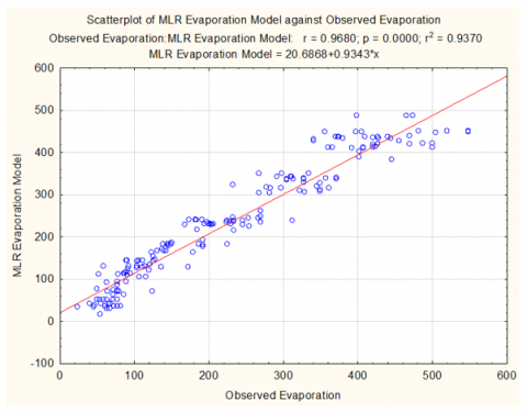
Model validation means verifying the validity of the developed models to ensure that can be used it with high efficiency under the same conditions to get accurate prediction results. For the model validation purposes, 280 dataset number (20% of the dataset) was used. The proportion of 20% of the dataset applied in this study for model validation is widely used and approved in many investigations. However, other studies, such as Almedeij [25] and Silval et al. [13] employed smaller percentages 17% and 15% respectively. The relationship between the observed and predicted evaporation regression model is presented (see Figure 3), suggesting that there is a strong correlation between observed and predicted values. The r and R2 values were calculated as 0.968 and 0.937 respectively.
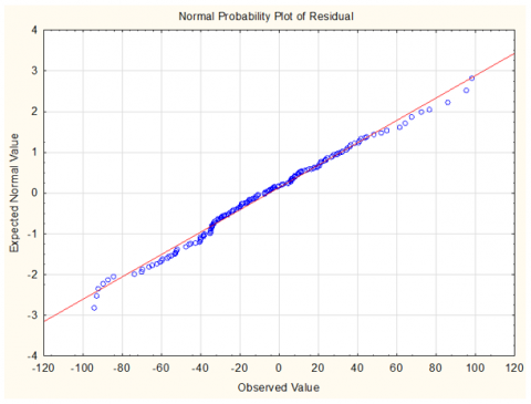
Figure 4 shows that the normal distribution of the residual satisfies the assumption of often made about normal distribution, residual distributions plot was approximately normal, an indication of adequate model fit.
Figure 3. Validation of MLR evaporation developed model
Figure 4. Normality of residual and equal of variance of residual
Performance indicators criteria were used to evaluate the accuracy of the MLR evaporation developed model (see Table 5).
Table 5. Performance Indicators for Evaporation validation model
|
Performance Indicators (PI) |
MLR evaporation developed Model |
|
R2 |
0.937 |
|
RMSE |
36.3 |
|
NAE |
0.123 |
|
MAPE |
17.83 |
|
NSE |
0.936 |
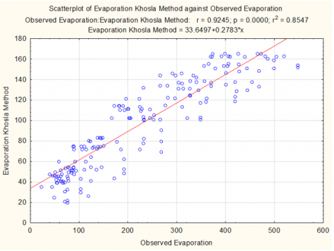
By comparing the MLR evaporation developed a model with the most common evaporation models commonly used in arid regions such as Kharufa and Khosla model. This model had been widely used by researchers to study evaporation and water balance modeling. Table 6 shows the performance indicators for the above models, the following inferences have been made. For MLR evaporation developed model R2 was 0.937 while Kharufa and Khosla model were 0.90 and 0.85 respectively. Thus, in terms of this indicator, MLR performed the best. Moreover, the values of the error measures, namely RMSE and NAE for MLR evaporation developed model were 36.3 and 0.123, Kharufa model 71.22 and 0.241 and Khosla model was and 173.7 and 0.581 respectively. Therefore, in terms of these two indicators, the MLR evaporation developed model performed the best. The remaining accuracy measures NSE and MAPE for MLR evaporation developed model were 0.936 and 17.83, Kharufa model 0.754 and 28.79 and Khosla model was 0.463 and 51.10 respectively. In terms of these two indicators, MLR performed the best.
Table 6. Comparison of performance between Evaporation MLR model and Kharufa and Khosla model
|
Performance Indicator |
Monthly Regression Evaporation model |
Kharufa model |
Khosla method |
|
R2 |
0.937 |
0.900 |
0.85 |
|
RMSE |
36.3 |
71.22 |
173.7 |
|
NAE |
0.123 |
0.241 |
0.581 |
|
MAPE |
17.83 |
28.79 |
51.10 |
|
NSE |
0.936 |
0.754 |
0.463 |
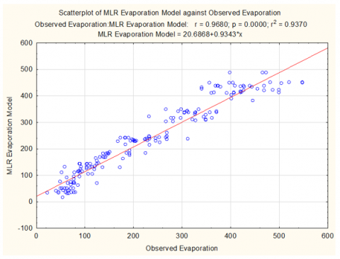
Figure 5. Scatter plot of observed dataset with MLR evaporation developed model using validation dataset
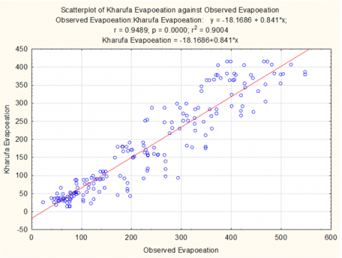
Figure 6. Scatter plot of observed dataset with Kharufa model using validation dataset
Figure 7. Scatter plot of observed dataset with Khosla model using validation dataset
Based on the foregoing, indicates that the results of performance indicators of the MLR developed evaporation model in the current study outperform all performance indicators and prove to be better than the aforementioned models (see Figure 5, Figure 6 and Figure 7).
The current study developed a monthly evaporation model using multiple linear regression suitable for the western area of Iraq (Horan Valley) in addition to its suitability for all arid regions. In this study, a new and accurate method was used to determine the variables that significantly affect evaporation prediction by using multiple linear regression (Enter method). Increasing the number of independent variables in the MLR will lead to an increase in the value of R2 even if some of these independent variables are not significant, and therefore the use of adjusted R2 will be more accurate. The relationship of E with two independent variables showed that the highest linear relationship between E with T and WS and T with SS which gives the adjusted R2 value which is 0.934 and 0.930 respectively, based on this high result conclude that these two variables have a significant effect on evaporation prediction and can be used it alone in the absence of other variables. The T, WS and SS is the best significant group for the prediction of evaporation. Furthermore, the relative humidity did not affect the predictive equation of evaporation. The results showed that the MLR evaporation developed model has proven its efficiency and its ability to predict evaporation and the superiority against the most important models are used for estimating the evaporation in arid areas. Stepwise and backward linear regressions have proven a suitable technique to develop prediction models for all hydrological applications parameters. The lack of available data and the difficulty of obtaining them in dry areas is one of the common problems in estimating evaporation values. Based on the results of this study, the use of multiple regression technique will be useful in future studies.
The authors would like to acknowledge the contribution of the University of Anbar (WWW.uoanbar.edu.iq) via their prestigious academic staff in supporting this research with all required technical and academic support and also the authors are grateful to the Meteorological Organization Seismology of Iraq (IMOS)-Climatological Division, for providing the relevant data of pan evaporation, temperature, relative humidity, wind speed and sunshine.
|
Abbreviation |
Description |
|
E |
Pan Evaporation |
|
IMOS |
Iraqi Meteorological Organization Seismology |
|
MAPE |
The Mean Average Percentage Error |
|
MLR |
Multiple Linear Regression |
|
MWBM |
Monthly Water balance Modelling |
|
NAE |
Normalized Absolute Error |
|
NSE |
Nash-Sutcliffe efficiency |
|
p |
P – value |
|
PI |
Performance Indicator |
|
R2 |
Coefficient of determination |
|
r |
Correlation Coefficient |
|
RMSE |
Root Mean Square Error |
|
RH |
Relative Humidity |
|
SE |
Standard Error |
|
SR |
Surface Runoff |
|
SLR |
Simple Linear Regression |
|
SS |
Sunshine |
|
STD |
Standard Deviation |
|
T |
Temperature |
|
VIF |
Variation inflation factor |
|
WS |
Wind Speed |
[1] Almedeij, J. (2016). Modeling pan evaporation for Kuwait using multiple linear regression and time-series techniques. American Journal of Applied Sciences, 13(6): 739-747. https://doi.org/10.3844/ajassp.2016.739.747
[2] Sammen, S.S. (2013). Forecasting of evaporation from Hemren reservoir by using artificial neural network. Diyala Journal of Engineering Sciences, 6(4): 38-33. https://doi.org/10.24237/djes.2013.06403
[3] Saud, A., Said, M.A.M., Abdullah, R., Hatem, A. (2014). Temporal and spatial variability of potential evapotranspiration in semi-Arid Region: Case study the valleys of Western Region of Iraq. International Journal of Engineering Science and Technology, 6(9): 653-660.
[4] Saud, A., Azlin, M., Said, M., Abdullah, R., Hatem, A. (2016). Investigation of water balance methods of Haqlan Basin in the western region of Iraq. World Appl. Sci. J., 34(5): 652-656. https://doi.org/10.5829/idosi.wasj.2016.34.5.16
[5] Atiaa, A.M., Abdul-Qadir, A.M. (2012). Using fuzzy logic for estimating monthly pan evaporation from meteorological data in Emara/South of Iraq. Baghdad Sci. J., 9(1): 133-140. https://doi.org/10.21123/bsj.9.1.133-140
[6] Kisi, O., Heddam, S. (2019). Evaporation modelling by heuristic regression approaches using only temperature data. Hydrological Sciences Journal, 64(6): 653-672. https://doi.org/10.1080/02626667.2019.1599487
[7] Majhi, B., Naidu, D. (2021). Pan evaporation modeling in different agroclimatic zones using functional link artificial neural network. Information Processing in Agriculture, 8(1): 134-147. https://doi.org/10.1016/j.inpa.2020.02.007
[8] Li, C.L., Shi, K.B., Yan, X.J., Jiang, C.L. (2021). Experimental analysis of water evaporation inhibition of plain reservoirs in inland arid area with light floating balls and floating plates in Xinjiang, China. Journal of Hydrologic Engineering, 26(2): 04020060. https://doi.org/10.1061/(asce)he.1943-5584.0002032
[9] Almawla, A.S. (2017). Predicting the daily evaporation in Ramadi city by using artificial neural network. Anbar Journal of Engineering Sciences, 7(2): 134-139.
[10] Balogun, C. (1974). The influence of some climatic factors on evaporation and potential evapotranspiration at Ibadan, Nigeria. Ghana Journal of Agricultural Science, 7: 45-49.
[11] Alsumaiei, A.A. (2020). Utility of artificial neural networks in modeling pan evaporation in hyper-arid climates. Water, 12(5): 1508. https://doi.org/10.3390/w12051508
[12] Li, R., Wang, C. (2020). Precipitation recycling using a new evapotranspiration estimator for Asian-African arid regions. Theoretical and Applied Climatology, 140(1): 1-13. https://doi.org/10.1007/s00704-019-03063-9
[13] da Silva, H.J., dos Santos, M.S., Junior, J.B.C., Spyrides, M.H. (2016). Modeling of reference evapotranspiration by multiple linear regression. Journal of Hyperspectral Remote Sensing, 6(1): 44-58. https://doi.org/10.5935/2237-2202.20160005
[14] Shirgure, P.S. (2012). Evaporation modeling with multiple linear regression techniques–A review. Scientific Journal of Review, 1(6): 170-182.
[15] Gallego-Elvira, B., Baille, A., Martín-Górriz, B., Martínez-Álvarez, V. (2010). Energy balance and evaporation loss of an agricultural reservoir in a semi-arid climate (south-eastern Spain). Hydrological Processes: An International Journal, 24(6): 758-766. https://doi.org/10.1002/hyp.7520
[16] Abou El-Magd, I.H., Ali, E.M. (2012). Estimation of the evaporative losses from Lake Nasser, Egypt using optical satellite imagery. International Journal of Digital Earth, 5(2): 133-146. https://doi.org/10.1080/17538947.2011.586442
[17] Abdullah, S.S., Malek, M., Mustapha, A., Aryanfar, A. (2014). Hybrid of artificial neural network-genetic algorithm for prediction of reference evapotranspiration (ET) in arid and semiarid regions. Journal of Agricultural Science, 6(3): 191. https://doi.org/10.5539/jas.v6n3p191
[18] De Bruin, H.A.R. (1978). A simple model for shallow lake evaporation. Journal of Applied Meteorology, 17(8): 1132-1134. https://doi.org/10.1175/1520-0450(1978)017<1132:asmfsl>2.0.co;2
[19] Abtew, W. (2001). Evaporation estimation for Lake Okeechobee in south Florida. Journal of Irrigation and Drainage Engineering, 127(3): 140-147. https://doi.org/10.1061/(ASCE)0733-9437(2001)127:3(140)
[20] Deswal, S. (2008). Modeling of evaporation using M5 model tree algorithm. Journal of Agrometeorology, 10(1): 33-38.
[21] Al-Mukhtar, M. (2021). Modeling the monthly pan evaporation rates using artificial intelligence methods: A case study in Iraq. Environmental Earth Sciences, 80(1): 1-14. https://doi.org/10.1007/s12665-020-09337-0
[22] Vallet-Coulomb, C., Legesse, D., Gasse, F., Travi, Y., Chernet, T. (2001). Lake evaporation estimates in tropical Africa (lake Ziway, Ethiopia). Journal of hydrology, 245(1-4): 1-18. https://doi.org/10.1016/S0022-1694(01)00341-9
[23] Gavin, H., Agnew, C.A. (2004). Modelling actual, reference and equilibrium evaporation from a temperate wet grassland. Hydrological Processes, 18(2): 229-246. https://doi.org/10.1002/hyp.1372
[24] Chang, F.J., Chang, L.C., Kao, H.S., Wu, G.R. (2010). Assessing the effort of meteorological variables for evaporation estimation by self-organizing map neural network. Journal of Hydrology, 384(1-2): 118-129. https://doi.org/10.1016/j.jhydrol.2010.01.016
[25] Almedeij, J. (2012). Modeling pan evaporation for Kuwait by multiple linear regression. The Scientific World Journal, 2012: 574742. https://doi.org/10.1100/2012/574742
[26] Cahoon, J.E., Costello, T.A., Ferguson, J.A. (1991). Estimating pan evaporation using limited meteorological observations. Agricultural and Forest Meteorology, 55(3-4): 181-190. https://doi.org/10.1016/0168-1923(91)90061-T
[27] Fennessey, N.M., Vogel, R.M. (1996). Regional models of potential evaporation and reference evapotranspiration for the northeast USA. Journal of Hydrology, 184(3-4): 337-354. https://doi.org/10.1016/0022-1694(95)02980-X
[28] Hanson, C.L. (1989). Prediction of class A pan evaporation in southwest Idaho. Journal of Irrigation and Drainage Engineering, 115(2): 166-171. https://doi.org/10.1061/(ASCE)0733-9437(1989)115:2(166)