Pratimakorn Hakaew | Piyapat Panmuang | Prakasit Prabpal | Chonlatee Photong*
© 2022 IIETA. This article is published by IIETA and is licensed under the CC BY 4.0 license (http://creativecommons.org/licenses/by/4.0/).
OPEN ACCESS
This paper is present an application of multi-frequency alternating current source that can be adjust the frequency from 1 Hz to 1 kHz for vertical electrical sounding (VES) on soil resistivity investigations. Researchers have used the four-point electrodes array method for resistivity method in laboratory and field trial of soil resistivity measurements. The result in laboratory found that in each frequency of current source has significate influence on the homogeneous soil resistivity. It was shown that the implemented equipment can be used to measure the soil resistivity as required. In field trial the soil resistivity was investigated by the implemented equipment feeding the rectangular wave current through two current electrodes on the subsurface soil which embedded in the non-homogeneous soil in the field work. The current source can be scaled and frequency adjusted at 50 Hz, 100 Hz, 200 Hz, 500 Hz and 1 kHz, respectively. The subsurface field have repeated tests 30 times in each frequency by compared with standard resistivity measurement equipment. The result found that the non-homogeneous apparent soil resistivity can be investigated and at the frequency of 100 Hz is close to the standard tool.
soil resistivity, sample soil, vertical electrical sounding, four-point electrodes arrangement, multi-frequency alternating current source
Soil specific resistivity is the soil property which has benefited for geophysical surveys where geophysicists use to find the available underground resources. The most popular are groundwater, petroleum oil and many minerals.
There are several methods of geophysical surveying for example the seismic, magnetic, electromagnetic, gravity, radioactivity and resistivity methods [1], of which the soil resistivity method is a geophysical survey method, standardized, unrestricted survey area, the survey operate on the top of subsurface soil without borehole, simple and rapid to survey, simple geophysical interpretation and easy to find surveying tools easy to use and cost-effective.
Soil resistivity is the parameter for groundwater exploration, construction, irrigation [2], lightning protection and agriculture for the following reasons [3-19]. Many researchers have studied for a long time in both theory and practice in many research areas [3-30]. G. Cosoli et al found that the resistivity measurement method can be applied for mortar and concrete elements [3], where various works supported this research [4-9]. Moreover, the soil resistivity can be used for grounding design [10-17] and agriculture [18]. The soil resistivity is the indicator of soil moisture, salinity, porosity, organic matter level, which can be used for precision farming applications [18]. The research for finding groundwater has also applied the soil resistivity to investigate for soil fertility and cultivation of grass for livestock [19, 20]. In Israel, M. Goldman used electrical methods to monitor seawater intrusions [21]. From the literature, we have seen that soil resistivity has been a good indicator for many applications. To date, soil resistivity is still an important parameter.
The resistivity method is used to measure soil resistivity this measurement method is commonly applied for direct current or alternating current feeding at frequencies as low as about 1 kHz in subsurface soil which is called “Vertical Electrical Sounding” (VES), where most of the time DC voltage source is applied. The voltage is very high range from 100 volts to the maximum voltage at about 600 volts, making the instrument used to measure expensive and the polarization was occured in each the two current electrodes which caused the soil resistivity measurement was inaccuracy. Therefore, in this research, we have designed an alternating current source that can be adjusted the frequency from 1 Hz to 1 kHz and used to supply electricity in form rectangular pulses to the ground which this operated can be prevent the polarization that will be occur at two current electrodes. Instead of a DC voltage source, the built alternative current source uses a lower voltage and is significantly cheaper. The experiment investigates the effect of the different frequency values of the current source that have influence to soil resistivity in the measurement. Each frequency is repeated 30 times. The percentage error is calculated to determine the soil resistivity measurement accuracy. The built-in soil resistivity meter was used to measure soil resistivity in the field against a standard meter. The basic theory is given, the experimental details are described.
Measuring and calculating the resistivity of materials (ρ1) is taken into account the length (l), cross-sectional area (A) and resistance of that material (R) as shown in Eq. (1).
$\rho_{1}=\frac{R A}{l}$ (1)
If the ratio between the cross-sectional area (A) and the length of the material is fixed as a constant ratio of k1 as shown in Eq. (2).
$k_{1}=\left(\frac{A}{l}\right)$ (2)
By substituting Eq. (2) to Eq. (1) and apply the Ohm’s law (R=V/I), Eq. (3) will be obtained.
$\rho_{1}=k_{1}\left(\frac{V}{I}\right)$ (3)
where, $\rho_{1}$ is the material resistivity (Ω.m), R is the material resistance (Ω), l is a material length (m), A is the cross-section area (m2), V is the applied voltage (volt), I is the current (Ampere).
The soil resistivity measurement method given by the four-point electrodes arrangement [1, 9] is shown in Figure 1. The four electrodes are embedded in the subsurface soil about 10-20 cm to ensure withstand positions as recommended in [1] (see Figure 3). Electrode spacing has the same distance for all four electrodes, which varies between 1-5 meters for this research investigation. Hence, the soil resistivity obtained from Eq. (4).
$\rho_{2}=k_{2}\left(\frac{\Delta v}{I(t)}\right)$ (4)
where, ρ2 is the soil resistivity (Ω.m), Δv is the potential difference from the measurement (volt), I(t) is the current from the current source (Ampere), k2=2πa and a is the electrode spacing (m).
Figure 1. The four-point electrodes array method diagram
In Figure 1, the alternating current source emits rectangular AC through current electrode terminals C1 and C2 into the ground as shown in Figure 2(a) and produces a potential field. Equipotential is formed around C1 and C2 the hemisphere is shaped as shown in Figure 2 (a), (b). The potential difference was measured at potential electrode terminals P1 and P2 with the same electrode spacing (a) between four electrodes by using the four-point electrodes array method [1, 9]; placing the four electrode rodes perpendicularly and firmly with the ground surface as shown in Figure 3.
(a)
(b)
Figure 2. The current flow and equipotential electric field distribution of the applied setup
Figure 2(a) shows a side view section of the path of the rectangular pulse current into the soil (current flow). Thus, the hemi-sphere equipotential is formed around the two current electrodes, while Figure 2(b) shows a top view current flow and equipotential [1]. It should be noted that this theoretical equipotential fields could be assumed only when sufficient electric current is ensured applying to the ground for particularly different electrode spacing tests; especially, when testing the resistivity for large area as recommended in [1].
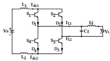
Figure 3. The equivalent circuit of soil specific resistivity measurement from implementation
Figure 3 shows the equivalent circuit of soil specific resistivity measurement equipment from implementation. The dc voltage from the battery (applied voltage) is supplied through the coil (L1, L2) that acts as the overlap time circuit to input of an electronic switching circuit as shown in Figure 4(a). An electronic switching circuit was operated in current source block diagram in Figure 3. The switching devices (S1, S2, S3 and S4) made from Insulated Gate Bipolar Transistor (IGBT), the switching circuit were alternating operation between S1, S3 and S2, S4 controlled by the reference current (Iref). From Figure 3 a signal generator circuit generates reference current in form rectangular shape and flow through a gate driver circuit to control the electronic switching devices. From this reason the output current of current source has the rectangular shape follow the current reference. A rectangular current is obtained through the output of the current source circuit with a duty cycle of 50%, as shown in Figure 4 (b). The frequency of the rectangular pulse current signal can be adjusted from 1 Hz to 1 kHz. The rectangular pulse current is supplied through the over current protection circuit and supplied to the current electrodes (C1, C2), respectively. The switching polarity of the electric current between positive and negative operating by the proposed electronic switching circuit (Figure 4(a)) can also solve the problem of polarization at the current electrodes; otherwise, the electrons and holes from the ground will recombine with the holes and electrons of the current electrodes, reduce electric field, and finally cause the inaccurate soil resistivity measurements.
(a)
(b)
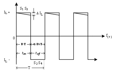
Figure 4. (a) An electronic switching circuit (b) rectangular pulse current from current source (I(t))
$D=\frac{t_{o n}}{t_{o n}+t_{o f f}}$ (5)
$L_{\min }=\frac{(1-D) R_{e q}}{2 f}$ (6)
$I_{L_{1,2}}=V_{L}\left[\frac{1}{R_{e q}} \pm \frac{(1-D)}{2 f L_{\min }}\right]$ (7)
When in Figure 4(a) Vs is the dc voltage from battery (volt), Idc1 and Idc2 are the direct current from battery (Ampere), VL is load voltage (volt), IL1 and Il2 are load current or the output rectangular pulse current from current source (Ampere) and in Figure 4(b) D is duty cycle (no unit), T is time or period (second), f is frequency (Hz), f=1/T, Lmin is the inductance of low-pass filter circuit (H), Lmin is equal Lf, and Req is the resistance of the switching circuit (Ω).
The soil resistivity measurement in each basement layer is based on a VES method. By releasing the AC rectangular pulse current flow into the basement at subsurface soil in the measurement site, the current will flow through the two outside electrode poles (current electrodes), which also provide benefit of polarization effect elimination as aforementioned in Section 2. The equipotential difference arising from the current flown through current electrodes can be obtained from the two inside electrode poles (potential electrodes). The variable parameters obtained from measurements such as the current from current source (I(t)), potential difference (Δv) and electrode spacing distance (a) can be calculated from Eq. (4).
From Eq. (4), the apparent soil resistivity obtained from measured have several values because the measurement procedure was expanded the distance of electrodes spacing on subsurface soil of distances 1m, 3m, and 5m, respectively. In each electrode spacing values can be obtained the difference values of apparent soil resistivity from Eq. (4). The geophysicists can be interpreted the geological exploration by plotting graph compared between the electrode spacing values versus apparent soil resistivity values. The depth of each difference apparent soil resistivity were indicated by the distance of each electrode spacing because the depth and the electrode spacing are the radius of hemi-spherical shape of equipotential in soil under measurement. Then, geophysicist can be interpreting in each layer of non-homogeneous soil.
In this research, there were two experimental sections: The laboratory experimental section and the field trial in field work site.
3.1 Laboratory experimental
For laboratory experimental site the sample soil used in the experiment was obtained by following the method of civil engineering by sifting the soil through standard sieve No. 4, No. 8, No. 16, No. 30, No. 50, No. 100 and No. 200, respectively, which results in clay or silt, either based on the plastic index obtained from the determination of soil flow or liquid limit value [2]. An Eq. (8) give the plastic index. By sifting the soil through the sieve, the homogeneous soil will be used as the sample soil used in the experiment. The reason for using the homogeneous soil in this research is because of the fact that the homogeneous soil used is the pre-analyzed soil (predictable value of the soil resistivity) for the laboratory purposes; otherwise, the possible metal or high insulation particles could be mixed with the tested soil and lead to less accurate results.
$P_{i}=L_{l}-P_{l}$ (8)
where, Pi>0.73(Ll-20) for clay, Pi<0.73(Ll-20) for silt, Pi is plastic index, Ll is the liquid limit and Pl is the plastic limit.
The soil resistivity measurement equipment was setup. The sample soil was packed in rectangular box case with size of 30x60x40 cm, which in this research will use silt as a sample soil. By using four-point electrodes array method, two current electrodes were buried to under the homogeneous sample soil surface of 10 cm depth. The two potential electrodes were buried at inner between two outer current electrodes as same as depth with a distance between the electrode spacing of 10cm. The soil resistivity can be determined by releasing the alternative rectangular current from multi-frequency current source flow into the basement of a homogeneous soil. The current will flow through two outer current electrodes under the surface of sample soil, where the readings were taken from the electrical alternating ammeter in the soil resistivity measurement equipment and recorded. The current that flowed underground with the hemisphere shape caused the electric potential to rise the poles of both electrodes from the surface depth in the subsoil have the hemisphere as well. The potential difference was measured with an ac voltmeter from measurement equipment setup at the potential electrodes embedded in the sample soil to a depth of 10cm. It can use the electric current from the ammeter (I(t)), the potential difference ($\Delta v$) from the ac voltmeter and electrode spacing (a) to calculate the apparent soi1 resistivity from Eq. (4). The experiment will adjust the frequency of the electricity discharged underground from 1 Hz to 1 kHz of 16 values such as 1 Hz, 2Hz, 3 Hz, 5 Hz, 7 Hz, 10 Hz, 20 Hz, 30 Hz, 50 Hz, 70 Hz, 100 Hz, 200 Hz, 300 Hz, 500 Hz, 700 Hz and 1 kHz, respectively. Then consider how each frequency affects the apparent soil resistivity and how much error is different in each frequency. Each frequency was repeated the same experiment 30 times to observe how each current frequency responds to the apparent soil resistivity value. In this work, the sample soil's humidity, laboratory temperature, and lighting were kept constant throughout the experimental period.
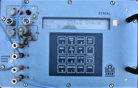
Figure 5. The standard resistivity meter model IRIS from IRIS Instruments France
3.2 Field trial for soil resistivity investigation
When the soil resistivity meter which implemented was used to measure the soil resistivity of the sample soil in the laboratory, the researchers used the soil resistivity meter was built to measure the soil resistivity in the field. The investigation procedure used the four-point electrodes array as same as the laboratory procedure and comparing it with the standard soil resistivity meter. Standard soil resistivity meter module IRIS is as shown in Figure 5. It is used to measure on a non-homogenous soil surface will expand the spacing of 1m, 3m and 5m, respectively. The four electrodes are made of copper rods with a diameter of 1.5 cm, a length of 40 cm, and the electrodes are buried 20 cm in the soil, as shown in Figure 3. The field measurements are as shown in Figure 6. The constructed and standard gauges are measured at the same subsurface soil, in which the electrodes are implanted at the same points in the same period. The distance between them is more than 20 minutes.
(a)
(b)
Figure 6. The soil resistivity measurement systems in this research
4.1 Laboratory
In laboratory experiments the results of experiments were shown in Table 1. It was found the results showed that the apparent soil resistivity varies with the current frequency applied to the soil by frequencies between 1 Hz-5 Hz. The average change of soil specific resistivity was 174.25 Ω.m -378.82 Ω.m, with frequencies higher than 5 Hz-700 Hz. The apparent soil specific resistivity was higher at an average of 741.84 Ω.m -1085.33 Ω.m. Then the soil resistivity began to decrease until an average of approximately 658.97 Ω.m at a frequency of 1 kHz. The results also indicated that the apparent soil specific resistivity measured at a frequency of 1 kHz gave the lowest error from 30 repetitions of measurements. The represented average of 1.0%, while the other frequency ranges an error of 1.6%-11.5% and the percentage of average error at a frequency of 100 Hz is 7.5%. The average value of apparent soil resistivity at all frequencies is 719.6 Ω.m and the percentage of average error at all frequencies is 6.41%. Figure 7 shows the average soil resistivity tested in the laboratory after 30 repetitions of each frequency using the rectangular pulses fed to the current electrodes. It found that the soil resistivity changed with the frequency value in each frequency, from which the error value is the lowest at 1% at a frequency of 1 kHz, as shown in Figure 8.
Table 1. Average soil resistivity from implemented instrument equipment in laboratory, electrode spacing is 10cm
|
Frequencies (Hz) |
Average soil resistivity (Ω.m) |
Average percentage error (%) |
|
1 2 3 5 7 10 20 30 50 70 100 200 300 500 700 1,000 |
174.25 242.86 289.4 378.82 754.91 1029.96 985.7 1085.33 993.81 945.17 813.62 803.55 870.73 741.84 74.55 658.97 |
2.5 1.6 1.8 2.1 7.9 9.9 5.4 7.8 7.4 9.1 7.5 11.5 6.1 10 10.9 1 |
Note: 1,000 Hz is equal to 1 kHz.
Figure 7. Graph shows the average apparent soil resistivity from the measurement respecting to frequency in laboratory
Figure 8. The percentage of error from laboratory
4.2 Field trial soil resistivity investigation
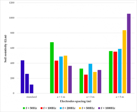
In a field trial, soil resistivity was measured with a built-in measuring instrument compared to a standard, where the measurement results are as shown in the Table 2 for standard. And Table 3 for the built instruments. In Figure 9. Soil resistivity measurements in the field at a distance of 1 m and 3 m showed that the values obtained from the built instruments were closest to that of the standard at 100 Hz. The spacing of the electrodes was 5 m. It found that current sources fed to an applied voltage as low as 24 V were unsuitable for non-homogeneous soil loads and the distance of electrode spacing was increasing to much. As a result, the current value is much lower, making the measured soil resistivity value much higher than the value measured by a standard meter following Eq. (4). Figure 9 shows the average apparent soil resistivity measured in the field to plot the graph at each frequency. The used frequencies were 50 Hz, 100 Hz, 200 Hz, 500 Hz and 1 kHz, respectively. The plotted against the average soil resistivity measured by a standard one. Apparent soil resistivity is obtained. From which at 100 Hz, the measurement results were closest to the standard soil resistivity meter. Figure 10 shows the average apparent soil resistivity values measured at each electrode spacing of 1m, 3m and 5m, respectively. The measured data was plotted against a standard soil resistivity at the same distance. It is close to the standard at the frequency of 100 Hz. While at a spacing distance of 5m, the measurement result is the average apparent soil resistivity. It is significantly different from the standard because the current source supplies current to the non-homogeneous subsurface soil and the distance of electrode spacing is increasing.
Table 2. Soil resistivity from standard meter in the field trial
|
Electrode spacing (m) |
Average soil resistivity (Ω.m) |
|
1 3 5 |
437.93 259.29 115.85 |
Table 3. Soil resistivity from implemented meter in the field trial
|
Frequencies (Hz) |
Average soil resistivity (Ω.m) (electrode spacing 1m) |
Average soil resistivity (Ω.m) (electrode spacing 3m) |
|
50 100 200 500 1,000 |
677.87 433.42 487.48 500.26 365.66 |
328.8 247.81 391.15 283.37 310.54 |
Note: 1,000 Hz is equal to 1 kHz.
Figure 9. The minimized graph of the values of average soil resistivity in each frequency range from measured
Figure 10. Graph of soil resistivity compares the standard and the constructed one, at different spacing distances
This work has purposed the application of a multi-frequency current source for solve polarization problem in the soil resistivity measurement system. Resistivity method and four-point electrodes array were used in the experiment procedures. Both results from the laboratory and field work found that the results from the homogeneous sample soil in laboratory was difference from the non-homogeneous soil in the field, but each result was good in the different way, such as in laboratory the percentage of error is lowest at the frequency of 1kHz, in field trial investigation has closed the standard tool at frequency of 100Hz. The problem of polarization at the current electrodes was solved by adjusting the current source frequency in measurement procedures from 1Hz to 1kHz. In the field work investigation at the electrode spacing of 5m can be solved by adapt the battery voltage up from 24V to 48-60V. In further research should be conducted by expanding the electrode spacing distance several times. Periodically, the experiment is repeated to determine which frequency value responds to the measurement or produces the most accurate and accurate measurement results. Alternatively, once the experiment has achieved the desired results, it is advisable to create an alternating current source of this value for VES. The most optimized frequencies are then applied to the soil in the actual field by comparison with another standard soil resistivity instrument. Further work can use this result to build a compact prototype resistivity measurement equipment at a frequency of 100Hz with an ac source to the soil contents.
This work is supported by Mahasarakham University, Institute of Vocational Education Northeastern Region 2, Sakonnakhon and Bureau of Groundwater Resources Region 10, Udonthani, Ministry of Natural Resources & Environment Bangkok, Thailand.
|
cm |
centimetre |
|
m |
metre |
|
m2 |
square metre |
|
$\Omega$ |
Ohm |
|
$\Omega$.m |
Ohm.metre |
|
V |
Volt |
|
A |
Ampere |
|
Hz |
Hertz |
|
kHz |
Kilohertz |
[1] Telford, W.M., Geldart, S., Sheriff, R. E., Keys, D.A. (1978). Applied geophysics. Cambridge University Press, England, 632-734. https://doi.org/10.1017/S0016756800050858
[2] Lambe, T.W., Whitman, R.W. (1979). Soil Mechanics, SI Version. John Wiley& Sons, New York, USA, 29-51. https://doi.org/10.1177/030913338100500325
[3] Cosoli, G., Mobili, A., Tittarelli, F., Revel, G.M., Chiariotti, P. (2020). Electrical resistivity and electrical impedance measurement in motar and concrete elements: A systematic review. Appl. Sci., 10(24): 9152. https://doi.org/10.3390/app10249152
[4] Azarsa, P., Gupta, R. (2017). Electrical resistivity of concrete for durability evaluation: A review. Advance in Materials Science and Engineering, 2017: 8453095. https://doi.org/10.1155/2017/8453095
[5] Liu, S.Y., Du, Y.J., Han, L.H., Gu, M.F. (2008). Experimental study on the electrical resistivity of soil-cement admixtures. Environment Geology, 54: 1227-1233. https://doi.org/10.1007/s00254-007-0905-5
[6] Mostafa, M., Anwar, M.B., Radwan, A. (2018). Application of electrical resistivity measurement as quality control test for calcareous soil housing and building. National Research Center (HBRCJ), 14(3): 379-384. https://doi.org/10.1016/j.hbrcj.2017.07.001
[7] Dahlin, T., Aronsson, P., Thornelof, M. (2014). Soil resistivity monitoring of an irrigation experiment. Near Surface Geophysics, 12(1): 35-44. https://doi.org/10.3997/1873-0604.2013035
[8] Tremsin, V.A. (2017). Real-time three-dimensional imaging of soil resistivity for assessment of moisture distribution for intelligent irrigation. Hydrology, 4(4): 54. https://doi.org/10.3390/hydrology4040054
[9] Wei, X., Ding, Z., Wu, J., Lui, B. (2013). Research on the high precision resistivity probe with four point- electrodes for marine sediments. Journal of Electronic Measurement and Instrument, 27(9): 810-816. https://doi.org/10.3724/sp.j.1187.2013.00810
[10] Androvitsaneas, V.P., Damianaki, K.D., Christodoulou, C.A., Gonos, I.F. (2020). Effect of soil resistivity measurement on the safe design of grounding systems. Energies, 13(12): 3170. https://doi.org/10.3390/en13123170
[11] Salam, M.A., Jen, K.M., Khan, A. (2011). Measurement and simulation of grounding resistance with two and four mesh grids. 2011 IEEE Ninth International Conference on Power Electronics and Drive Systems. https://doi.org/10.1109/peds.2011.6147248
[12] Ma, J., Dawalibi, F.P. (2020). Analysis of grounding systems in soils with finite volumes of different resistivities. IEEE Transactions on Power Delivery, 17(2): 596-602. https://doi.org/10.1109/61.997944
[13] Visacro, S., Alipio, R., Vale H.M., Pereira, C. (2011). The response of grounding electrodes to lightning currents: The effect of frequency-dependent soil resistivity and Permittivity. IEEE Transactions on Electromagnetic Compatibility, 53(2): 401-406. https://doi.org/10.1109/temc.2011.2106790
[14] Ghourab, M.E. (1996). Evaluation of earth resistivity for grounding systems in non-uniform soil structure. European Transactions on Electrical Power, 6(3): 195-200. https://doi.org/10.1002/etep.4450060309
[15] Alipio, R., Visacro, S. (2013). Frequency dependence of soil parameters: Effect on the lightning response of grounding electrodes. IEEE Transaction on Electromagnetic Compatibility, 55(1): 132-139. https://doi.org/10.1109/temc.2012.2210227
[16] Sima, W., Liu, S., Yuan, T., Luo, D., Wu, P., Zhu, B. (2015). Experimental study of the discharge area of soil breakdown under surge current using x-ray imaging technology. IEEE Transactions on Industry Applications, 51(6): 5343-5351. https://doi.org/10.1109/tia.2015.2448615
[17] Cayka, D., Mora, N., Rachidi, F. (2014). A comparison of frequency-dependentsoil models: Application to the analysis of grounding systems. IEEE Transactions on Electromagnetic Compatibility, 56(1): 177-187. https://doi.org/10.1109/temc.2013.2271913
[18] Unal, I., Kabas, O., Sozer, S. (2020). Real-time electrical resistivity measurement and mapping platform of the soils with an autonomous robot for precision farming application. Sensors, 20(1): 251. https://doi.org/10.3390/s20010251
[19] Mohamaden, M.I.I., Abuo, S.S., Gamal, A.A. (2009). Geo-electrical survey for groundwater exploration at the Asuit Governorate, Nile Valley, Egypt. JKAU. Mar. Sci., 20: 91-108. https://doi.org/10.4197/mar.20-1.7
[20] Umeh, V.O., Chukwudi, C.C., Okonkwo, A.C. (2014). Groundwater exploration of Lokpaukwu, Abia State Southeastern Nigeria, using electrical resistivity method. International Research Journal of Geology and Mining (IRJGM), 22276-6618, 4(3): 76-83. https://doi.org/10.14303/irjgm.2014.019
[21] Goldman, M., Gilad, D., Ronen, A., Melloul, A. (1991). Mapping of seawater intrusion into the coastal aquifer of Israel by the time domain electromagnetic method. Geoexploration, 28(2): 153-174. https://doi.org/10.1016/0016-7142(91)90046-f
[22] Datsios, Z.G., Mikropoulos, P.N., Karakousis, I. (2017). Laboratory characterization and modeling of dc electrical resistivity of sandy soil with variable water resistivity and content. IEEE Transactions on Dielectrics and Electrical Insulation, 24(5): 3063-3072. https://doi.org/10.1109/tdei.2017.006583
[23] Zhou, M., Wang, J., Cai, L., Fan, Y., Zheng, Z. (2015). Laboratory investigations on factors affecting soil electrical resistivity and the measurement. IEEE Transactions on Industry Applications, 51(6): 5358-5365. https://doi.org/10.1109/tia.2015.2465931
[24] Nor, N.M., Haddad, A., Griffiths, H. (2006). Performance of earthing system of low resistivity soils. IEEE Transactions on Power Delivery, 21(4): 2047-2049. https://doi.org/10.1109/tpwrd.2006.874656
[25] Ramos-Leanos, O., Uribe, F.A., Valcarcel, L., Hajiaboli, A., Franiatte, S., Dawalibi, F. (2020). Nonlinear electrode arrangements for multilayer soil resistivity measurements. IEEE Transactions on Electromagnetic Compatibility, 62(5): 2148-2155. https://doi.org/10.1109/temc.2020.2970149
[26] Ferreira, Q. de C.G., Bacellar, L.A.P., Vian, J.H.M. (2021). Evaluation of soil moisture by electrical resistivity in oxisols of the Central Brazilian Savanna. Geoderma Regional, 26: e00408. https://doi.org/10.1016/j.geodrs.2021.e00408
[27] Nielson, T., Bradford, J., Piece, J., Seyfried, M. (2021). Soil structure and soil moisture dynamics inferred from time-lapse electrical resistivity tomography. CATENA, 207: 1005553. https://doi.org/10.1016/j.catena.2021.105553
[28] Alsharari, B., Olenko, A., Abuel-Naga, H. (2020). Modeling of electrical resistivity of soil base on geotechnical properties. Expert Systems wth Applications, 141: 112966. https://doi.org/10.1016/j.eswa.2019.112966
[29] Tang, L., Wang, K., Jin, L., Yang, G., Jia, H., Taoum, A.A. (2018). Resistivity model for testing unfrozen water content of frozen soil. Cold Region Science and Technology, 153: 55-63. https://doi.org/10.1016/j.coldregions.2018.05.003
[30] Salam, Md. A., Rahman, Q.M., Ang, S.P., Wen, F. (2017). Soil resistivity and ground resistance for dry and wet soil. J. Modern Power Systems and Clean Energy, 5: 290-297. https://doi.org/10.1007/s40565-015-0153-8