Jielong Hu | Pingyi Wang* | Jie Zhang | Meili Wang | Yafei Chen | Congcong Zhao
© 2020 IIETA. This article is published by IIETA and is licensed under the CC BY 4.0 license (http://creativecommons.org/licenses/by/4.0/).
OPEN ACCESS
To disclose the turbulence features near a permeable spur dike, this paper measures the three-dimensional (3D) instantaneous velocity at different vertical lines and depths around the permeable spur dike through acoustic Doppler velocimetry (ADV). The relative turbulence intensity and Reynolds stress were calculated for each measuring point, and the distribution features of different turbulence structures were analyzed along the water depth. Experimental results show that: within the length of the dike, the turbulence intensity and Reynolds stress in the downstream of the dike are much greater than those in the upstream. In the downstream of the dike, the turbulence intensity in the root and body regions peaks in the dike crest layer, but that at other positions minimizes in that layer (but peaks on the water surface or river bottom). In the upstream, ejection and sweeping are the dominant turbulence structures; the two structures also dominate near the free layer at the bottom in the downstream; outward and inward interactions dominate near the dike crest layer in the downstream.
permeable spur dike, turbulence intensity, turbulence structure, turbulent kinetic energy, quadrant analysis
As a waterway regulation structure, the spur dike has been widely used to divert water flow, protect river banks, and restore waterway ecology [1, 2]. The turbulence has a great impact on the erosion of river bottom and the life of aquatic organisms. To fully understand the influence of turbulence around a spur dike, it is necessary to thoroughly analyze the turbulence features.
The structure and flow mechanism of the turbulence around spur dike have been extensively studied through flume experiments. For example, Rajaratnam and Nwachukwu [3] conducted flume experiments to ascertain the structure of turbulence near the spur dike, using the model of the three‐dimensional (3D) turbulent boundary layer. Ohmoto et al. [4] experimentally clarified the momentum exchange between main flow and the spur dike regions, revealing the obvious correlation between the water surface oscillation around the spur dike and velocity fluctuation. Jeon et al. [5] investigated the flow structure and turbulence mechanism around a non-submerged spur dike. Koken and Gogus [6] examined the different shear stresses and pressures on river bottom at three different spur dike lengths. Mehraein et al. [7] analyzed the turbulent kinetic energies and Reynolds stresses at different positions near the bottom of straight spur dike. Gu et al. [8] carried out flume experiments to observe the properties of turbulence structures on permeable and impermeable dikes. Through lab experiments, Hasegawa et al. [9] found that permeable pile spur dike can reduce the longitudinal velocity and turbulence intensity in the near-bank area.
Some scholars measured the 3D flow fields and turbulence features around the spur dike through acoustic doppler velocimetry (ADV). For instance, Duan et al. [10-12] captured the turbulence intensity and Reynolds stress of spur dikes by the ADV, and tackled the changes of turbulent states before and after the formation of the scour hole, including outward interaction, ejection, inward interaction, and sweeping. With the aid of the ADV, Jeon and Kang [13] obtained the 3D instantaneous velocities of the 3D turbulences around a spur dike, and derived the turbulence stresses from the obtained data.
Some other scholars explored the turbulence features around spur dikes through numerical simulation and theoretical analysis. Soulsby and Dyer [14], Keshavarzy and Ball [15], and Marchioli and Soldati [16] determined the correlations between the scour and near-bed turbulence parameters by means of quadrant analysis and triple correlations. Nikora and Goring [17], and Nezu [18] formulated the relations of velocity, turbulence intensity, and Reynolds stress after measuring the turbulence intensity and kinetic energy. Cui and Zhang [19] combined the k-epsilon (ε) model and the wall function into a new model, simulated the flow field around spur dike with free surface, and calculated the turbulent kinetic energy and its dissipation rate. Zhang [20] developed a 3D non-linear k-ε model to simulate the turbulence in the local scour hole around a single non-submerged spur dike. Acharya and Duan [21] adopted the renormalization group (RNG) k-ε model to simulate the turbulence field around spur dikes. Kang et al. [22] simulated the turbulence fields around multiple-arm instream structures, using the large-eddy simulation (LES) model, which solves the 3D Navier-Stokes equations, and the curvilinear immersed boundary (CURVIB) method.
To sum up, many experiments and simulations have been conducted to reveal the turbulence characteristics around spur dikes. However, the experimental studies have two common defects: the measuring points are close to the scour hole or the river bottom; the turbulent data are often collected from one horizontal plane, failing to reflect the turbulence features along the water depth. As for the simulation analyses, the turbulence features (e.g. turbulence intensity and Reynolds stress) obtained by most simulation models lack support from measured data, which dampens the simulation accuracy and applicability. What is worse, the previous studies on the turbulence features around spur dikes mostly emphasize on solid spur dikes, paying little attention to permeable spur dikes.
This paper measures the flow field around a permeable spur dike, which is installed at an open channel, through Nortek Vectrino Plus ADV. The time history of 3D velocities at all measuring points around the dike was recorded. Based on the measured data, the variation rules of turbulence intensity at different parts of the dike were analyzed along the water depth. In addition, the turbulence structure was discussed through quadrant decomposition. In this way, the authors quantified the turbulent Reynolds stress contribution of different flow regimes, and disclosed the relationship between Reynolds stress and turbulent kinetic energy.
Our experiments were conducted in a 30m-long and 3m-wide straight open-channel flume with zero bed slope and concrete sidewalls and bottom. The water was piped into the flume from an underground reservoir. The depth and surface drop of water were controlled by a tailgate. The flume system is shown in Figure 1.
Figure 1. The flume system
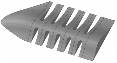
Looking in the downstream direction, a permeable spur dike was installed perpendicularly to the left sidewall at 18m away from the inlet. The body curve of the dike was designed based on the WES curve of overflow weir. The permeable spur dike is 135cm long, 72cm wide and 15cm high. Each member of the dike has an 3cm-wide arch hole, and a water permeability of 17.6%. The curve of the dike body and the stereogram of the dike are shown in Figure 2 and Figure 3, respectively.
Figure 2. The curve of dike body (unit: cm)
Figure 3. The stereogram of permeable spur dike
During the experiments, the 3D instantaneous flow velocities were collected by a Nortek ADV (Vectrino+) equipped with a side-looking head. For every experiment, the velocity rate was set to 1.0m/s, the sampling rate was maintained at 100Hz, and the data accuracy was realized at 0.001m/s. The data accuracy is positively correlated with the signal correlation coefficient (COR), and the signal-to-noise ratio (SNR). The COR and SNR of the measured data were greater than 90% and 18dB, respectively.
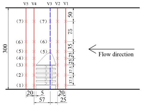
The ADV was fixed on an instrument carriage, which was mounted on horizontal steel rails and moved along the flume on wheels. In addition, the vertical error, longitudinal accuracy, and transversal accuracy of the probe were set to 1mm, 5mm, and 5mm, respectively. A total of five cross-sections was measured. Each cross-section has seven vertical profiles, except profile V3. On each vertical profile, 17 measuring points were arranged at the interval of 1cm. Figures 4 and 5 illustrate the arrangement of measuring points.
In Figure 4, profiles V1 and V2 are located 5cm and 25cm in the upstream of the dike, respectively; profile V3 is the axis of the dike; profiles V4 and V5 are located 5cm and 25cm in the downstream of the dike, respectively. The seven profiles are 15cm away from the root, middle, and the head of the dike, 15cm away from the root and middle of dike head, 40cm in front of the dike head, and 50cm away from the right bank of the flume.
The flow direction, longitudinal direction, and vertical direction were taken as axes X, Y, and Z, respectively. In addition, the flow rate (Q) is 0.142m3/s, the water depth (H) is 20cm, the hydraulic gradient (J) is 0.0006, the dike height (h) is 15cm, the Reynolds number (Re) is 47,333, and the Froude number (Fr) is 0.169.
Figure 4. The planar layout of measuring points (unit: cm)
Figure 5. The vertical layout of measuring points (unit: cm)
The proposed permeable spur dike can regulate the waterway and restore the ecology. On the one hand, the dike slows down the erosion of sediment around the dike; on the other hand, the dike provides aquatic organisms, especially fish, with small habitats and migration channels. It is important to analyze the turbulence intensity and structure near the dike, because the two factors directly bear on the movement and transportation of sediment [23], as well as the behaviors of fish, e.g. movement, spawning, and migration [24].
3.1 Turbulence intensity
Turbulence intensity (σ) indicates the intensity of the velocity pulsation in the water flow:
${{\sigma }_{u}}={{\left( {{n}^{-1}}\sum\limits_{i=1}^{n}{u_{i}^{\prime 2}} \right)}^{1/2}}$ (1)
${{\sigma }_{V}}={{\left( {{n}^{-1}}\sum\limits_{i=1}^{n}{V_{i}^{\prime 2}} \right)}^{1/2}}$ (2)
${{\sigma }_{W}}={{\left( {{n}^{-1}}\sum\limits_{i=1}^{n}{w_{i}^{\prime 2}} \right)}^{1/2}}$ (3)
where, σu, σv, and σw are turbulence intensities in X, Y, and Z directions, respectively; $u_{i}^{\prime}, v_{i}^{\prime}$, and $w_{i}^{\prime}$ are the fluctuating velocities in X, Y, and Z directions, respectively; n is the sample size.
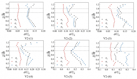
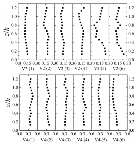
To disclose the rule of turbulence intensity along the water depth, the dimensionless turbulence intensity (σ/U0) distribution at each point of profiles V2 and V4 were analyzed under different submersion degrees (z/h) (Figure 6):
$U_{0}=Q / H B$ (4)
Under the submergence degree of 1, the height of the measuring point equals that of the dike; under the submergence degree of 0.8, the measuring point lies right on the top of the dike hole. In addition, the positions of z/h>1, 0.8<z/h<1, and z/h<0.8 were defined as the free layer, dike crest layer, and dike body layer, respectively.
As shown in Figure 6, on the same vertical line, the variation law of 3D turbulence intensity was basically the same along water depth, and $\sigma_{v}$ was smaller than $\sigma_{u} \text { and } \sigma_{w}$. Section V2 is located at the upstream of the dike, and the water flow is relatively stable.
In the vertical direction, with the growing submersion degree, the turbulence intensity first decreased and then increased. With the decline in submersion degree, the turbulence intensity decreased in the free layer, but changed suddenly in the dike crest layer. Below the dike crest layer, the turbulence intensity increased with the falling submergence degree. The minimum turbulence intensity appeared in the dike crest layer, while the maximum turbulence intensity was observed on the water surface or river bottom. There was not much difference between the two values.
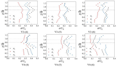
On profile V4 lies in the downstream of the dike. The variation in turbulence intensity behind the dike was complicated by the dike permeability. At v4-(1) and v4-(2), turbulence intensity peaked at z/h=0.8. With the decline in submersion degree, the turbulence intensity decreased in the free layer, but increased continuously across the dike crest layer. This rise of turbulence intensity is attributable to the fact that: the water flow in the dike hole spreads at the outlet, forming a hydraulic jump, and interacts with the falling water flow over the dike top to produce severe turbulence. Within 0.5<z/h<0.8, the turbulence intensity decreased with submersion degree. From z/h=0.5 to the bottom, the turbulence became increasingly intense. Overall, the variation of turbulence intensity at other positions of profile V4 is similar to that of profile V2.
To further clarify the variation in turbulence intensity at different positions of the dike, the authors compared the turbulence intensities of profiles V2 and V4. Considering the similarity in the variation of turbulence intensity and the fact that σu and σw are obviously greater than σv, only the σu at different positions of the dike was analyzed in details (Figure 7).
As shown in Figure 7, the turbulence intensity in the downstream of the dike was generally twice that in the upstream, except in V2-(6) and V4-(6), which are 40cm from the right of the dike head. In the main channel of the river, the dike has less influence on the water flow. That is why V2-(6) and V4-(6) have little difference in turbulence intensity.
Figure 6. The distribution of 3D turbulence intensity
Figure 7. The σu distribution at different positions
3.2 Turbulence structure
3.2.1 Quadrant analysis
Quadrant analysis is a classic, stable, and popular way to analyze turbulence structure [25, 26]. The quadrant analysis of Reynolds stress was conceptualized by Lu and Willmarth [27] to examine the shear stress features on the outer boundary of the viscous bottom of turbulence. Since then, this approach has been widely applied to study the turbulence around spur dikes [28, 29].
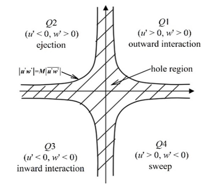
Quadrant analysis aims to distribute instantaneous pulsation velocity (u', w') in the four quadrants of the plane coordinate system (Q1, Q2, Q3 and Q4), and obtain the corresponding Reynolds stress contribution Si, M in each quadrant (Figure 8). In the first quadrant Q1 (u'>0, w'>0), the high-speed fluid moves away from the bed surface, belonging to the outward interaction state; In the second quadrant Q2 (u'<0, w'>0), the low-speed fluid moves away from the bed surface, belonging to the ejection state; In the third quadrant Q3 (u< 0, w'<0), the low-speed fluid moves towards the bed surface, belonging to the inward interaction state; In the fourth quadrant Q4 (u'>0, w'<0), the high-seed fluid moves towards the bed surface, belonging to the sweeping state.
Figure 8. The four quadrants and the hole region
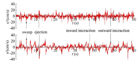
From the time distribution of pulsation velocities u' and w', it is clear that various flow states alternated with the elapse of time. The time distribution of pulsation velocity at vertical line V4-(5) in dike crest layer (z/h=1) was selected for detailed analysis. Under the above conditions of state identification, the four flow states were observed clearly in Figure 9.
Figure 9. The time distribution of pulsation velocity
The hole region [27], that is, the shaded part in Figure 8, refers to the region bounded by four hyperbolas $\left|u^{\prime} w^{\prime}\right|=M\left|\overline{u^{\prime} w^{\prime}}\right|$, where M is the size of the hole region. Under different M values, the contribution of each flow state to Reynolds stress Si,M (i=1,2,3,4) can be calculated by:
${{S}_{i,M}}=\frac{1}{T}\int_{0}^{T}{{{C}_{i,M}}}(t){{u}^{\prime }}(t){{w}^{\prime }}(t)dt$ (5)
If $\left|\mathrm{u}^{\prime}(\mathrm{t}) \mathrm{w}^{\prime}(\mathrm{t})\right|>\mathrm{M}\left[\overline{\mathrm{u}^{\prime} \mathrm{w}^{\prime}}\right] \text { and }\left[u^{\prime}(t) w^{\prime}(t)\right]$ fall in the Qi quadrant, Ci,M=1; otherwise, Ci,M=0.
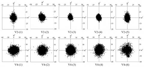
All instantaneous pulsation velocities are counted when M=0. Next, the turbulence distribution of each vertical line of profiles V2 and V4 was analyzed to clearly understand the distribution of pulsation velocities (u' and w') in each quadrant (Figure 10).
As shown in Figure 10, the transverse pulsation velocity (u') and vertical fluctuating velocity (w') of the flow in the upstream of the dike were both smaller than those in the downstream. This echoes with the finding in subsection 3.1 that the turbulence intensities in the downstream were greater than those in the upstream.
Figure 10. The distribution of pulsation velocities $\left(u^{\prime}, w^{\prime}\right)$
In the scoure hole, the sediment partciles are lifted by sweeping and ejection flows (u'>0, w'<0; u'<0, w'>0), and rotated by the transverse pulsation velocity [28]. Therefore, ejection (Q2) and sweeping (Q4) dominate the total sample, and require further analysis.
The vertical pulsation velocities (w') of the profile in the upstream of the dike were greater than the transverse pulsation velocity (u'). The ratios of (K2+K4)/(K1+K3) in V2-(1),V2-(2),V2-(3),V2-(4), and V2-(5) were 1.06, 1.24, 1.41, 1.39, and 1.07, respectively, where Ki is the percentage of Si,0 in the total sample. Overall, the turbulence structure in the upstream of dike do not result in severe sediment scour.
In addition, transverse pulsation velocities (u') of the profile in the downstream of the dike were greater than the vertical pulsation velocity (w'). The ratios of (K2+K4)/(K1+K3) in V4-(1), V4-(2), V4-(3), V4-(4), and V4-(5) were 0.9, 0.94, 1.01, 1.06, and 1.08, respectively. Thus, it is difficult for the sediment to accmulate at the dike root. This explains the relatively slight scour at that position. Moreover, the sediment at other positions are susceptible to accumulation and transporting to the downstream. As a result, the downstream of the dike suffers serious scour.
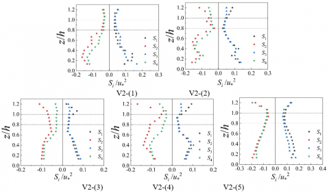
To understand the distribution of different turbulence structures along water depth, the relationship between Reynolds stress contribution and submergence degree was quantified carefully. Under M=0, the Reynolds stress contribution was nondimensionalized by the square of frictional velocity $S_{i} / u *^{2}$ :
${{u}_{*}}=\sqrt{gHJ}$ (6)
where, H=19cm is water depth; J=0.0006 is the hydraulic gradient.
Figure 11. The relationship between the Reynolds stress contribution and submergence degree
Figure 11 shows the relationship between the Reynolds stress contribution and the submergence degree.
As shown in Figure 11, on every vertical line in the upstream and downstream of the dike, the four turbulence structures (Qi) changed by basically the same law along the water depth. The Reynolds stress contribution $\mathrm{S}_{\mathrm{i}}$ of the upstream profile V2 of the spur dike was smaller than that of the downstream profile V4.
From water surface to river bottom, the turbulence structure on each vertical line of profile V2 was dominated by ejection (Q2) and sweeping (Q4). Besides, S2 was the larget contribution. The $\mathrm{S}_{\mathrm{i}}$ on V2-(1) (dike root) increased continuously from the water surface to the river bottom.
At other positions, Si decreased first and then increased with the growing submergence degree. The largest contribution appeared on the water surface or the river bottom, while the smallest emerged in the dike crest layer.
The downstream profile V4 exhibited more complex turbulence structures. Ejection (Q2) and sweeping (Q4) dominated the turbulence structure bear the free layer and the bottom, while outward interaction (Q1) and inward interaction (Q3) dominated near the dike crest layer. The greatest contribution appeared in the dike crest layer. However, there was no obvious law in the variation of Si with water depth. A possible reason is the mixing and interaction of the backflow of water behind the dike, the flow around the dike head, the overflow over the dike crest, and the jet flow from dike body.
3.3 Reynolds stress and turbulent kinetic energy
Turbulent kinetic energy mirrors the turbulent state of water flow, and manifests the energy loss of water flow caused by turbulence. As a strong mixed water current, turbulence signifcantly promotes the growth and spawning of fishes [30]. In open channels, ejection (S2) and sweeping (S4) are the main sources of turbulent energy. They exist as the most important largescale structure in open channel turbulence, and boast a gigantic amount of energy from wall to free water surface [31]. Here, the Reynolds stress contribution is nondimensionalized by the frictional velocity $E / u *^{2}$ :
$E=\frac{1}{2}\left( u_{i}^{\prime 2}+w_{i}^{\prime 2} \right)$ (7)
Figure 12 illustrates the relationship between S2, S4 and turbulent kinetic energy.
Figure 12. The relationship between Reynolds stress and turbulent kinetic energy
As shown in Figure 12, the data points formed an increasing curve, and the R2 of the fitting formula stood at 0.91, suggesting the good correlation of the formula. Although the distribution of the points was relatively scattered after >1.0, the change trend remained consistent. Therefore, ejection (S2) and sweep (S4) states have consistent effects on turbulent kinetic energy.
The purpose of this research is to disclose the turbulence features of the water flow near the permeable spur dike. For this purpose, physical experiments were carried out to capture the changes of the turbulence intensity and structure along the water depth around the dike. The main conclusions are as follows:
(1) On the same vertical line, the 3D turbulence intensities exhibit basically the same change trend along the water depth; the longitudinal turbulence intensity σvis smaller than the lateral turbulence intensity σu and the vertical turbulence intensity σw. Within the length of the dike, the turbulence intensity in the downstream is roughly twice that in the upstream. The water flows in the main channel in the up- and downstream of the dike have virtually the same turbulence intensity.
(2) In the upstream of the dike, the turbulence intensity minimizes in the dike crest layer, and maximizes at the water surface or river bottom. In the downstream of the dike, the turbulence intensity peaks at z/h=0.8 at the root and body of the dike; the turbulence intensity follows the same trend in other positions as that in the upstream.
(3) On the same vertical line, the four turbulence structures, namely, ejection, sweeping, outward interaction, and inward interaction, obey basically the same law along the water depth; the Reynolds stress in the upstream of the dike is smaller than that in the downstream.
(4) Ejection and sweeping are the dominant turbulence structures in the upstream of the dike; ejection makes the greatest Reynolds stress contribution. The Reynolds stress is relatively large on the water surface or the river bottom. By contrast, the Reynolds stress is the smallest in the dike crest layer. In the downstream of the dike, ejection and sweeping dominate the turbulence near the free layer and the bottom. The outward and inward interactions are dominant near the dike crest layer. In addition, the Reynolds stress contribution peaks in the dike crest layer.
(5) Ejection and sweeping are the main sources of turbulent energy. There is a good correlation between turbulent kinetic energy and Reynolds stress.
This work was supported by National Key Research and Development Projects of China (Grant No.: 2016YFC0402106; 2018YFB1600403), and Youth Fund of Chongqing Municipal Education Commission (Grant No.: 2020719051). Our thanks also go to Chengyu Yang for the assistance on the experiments.
[1] Huang, T., Lu, Y., Liu, H. (2019). Effects of spur dikes on water flow diversity and fish aggregation. Water, 11(9): 1822. https://doi.org/10.3390/w11091822
[2] Muste, M., Yu, K., Fujita, I., Ettema, R. (2005). Two-phase versus mixed-flow perspective on suspended sediment transport in turbulent channel flows. Water Resources Research, 41(10): 1-22. https://doi.org/10.1029/2004WR003595
[3] Rajaratnam, N., Nwachukwu, B.A. (1983). Flow near groin-like structures. Journal of Hydraulic Engineering, 109(3): 463-480. https://doi.org/10.1061/(ASCE)0733-9429(1983)109:3(463)
[4] Ohmoto, T., Hirakawa, R., Koreeda, N. (2002). Effects of water surface oscillation on turbulent flow in an open channel with a series of spur dikes. In Hydraulic Measurements and Experimental Methods 2002, pp. 1-10. https://doi.org/10.1061/40655(2002)108
[5] Jeon, J., Lee, J.Y., Kang, S. (2018). Experimental investigation of three‐dimensional flow structure and turbulent flow mechanisms around a nonsubmerged spur dike with a low length-to-depth ratio. Water Resources Research, 54(5): 3530-3556. https://doi.org/10.1029/2017WR021582
[6] Koken, M., Gogus, M. (2015). Effect of spur dike length on the horseshoe vortex system and the bed shear stress distribution. Journal of Hydraulic Research, 53(2): 196-206. https://doi.org/10.1080/00221686.2014.967819
[7] Mehraein, M., Najibi, S.A., Ghodsian, M. (2014). Location effect on near bed flow structure around a straight spur dike. In Proceeding of 9th International Symposium on Ultrasonic Doppler Methods for Fluid Mechanics and Fluid Engineering, pp. 173-176.
[8] Gu, Z.P., Akahori, R., Ikeda, S. (2011). Study on the transport of suspended sediment in an open channel flow with permeable spur dikes. International Journal of Sediment Research, 26(1): 96-111. https://doi.org/10.1016/S1001-6279(11)60079-6
[9] Hasegawa, Y., Nakagawa, H., Takebayashi, H., Kawaike, K. (2020). Three-dimensional flow characteristics in slit-type permeable spur dike fields: Efficacy in riverbank protection. Water, 12(4): 964. https://doi.org/10.3390/w12040964
[10] Duan, J.G. (2009). Mean flow and turbulence around a laboratory spur dike. Journal of Hydraulic Engineering, 135(10): 803-811. https://doi.org/10.1061/(ASCE)HY.1943-7900.0000077
[11] Duan, J.G., He, L., Fu, X., Wang, Q. (2009). Mean flow and turbulence around experimental spur dike. Advances in Water Resources, 32(12): 1717-1725. https://doi.org/10.1016/j.advwatres.2009.09.004
[12] Duan, J., He, L., Wang, G., Fu, X.D. (2011). Turbulent burst around experimental spur dike. International Journal of Sediment Research, 26(4): 471-523. https://doi.org/10.1016/S1001-6279(12)60006-7
[13] Jeon, J., Kang, S. (2016). Flume experiments for turbulent flow around a spur dike. Journal of Korea Water Resources Association, 49(8): 707-717. https://doi.org/10.3741/JKWRA.2016.49.8.707
[14] Soulsby, R.L., Dyer, K.R. (1981). The form of the near-bed velocity profile in a tidally accelerating flow. Journal of Geophysical Research: Oceans, 86(C9): 8067-8074. https://doi.org/10.1029/JC086iC09p08067
[15] Keshavarzy, A., Ball, J.E. (1997). An analysis of the characteristics of rough bed turbulent shear stresses in an open channel. Stochastic Hydrology and Hydraulics, 11(3): 193-210. https://doi.org/10.1007/BF02427915
[16] Marchioli, C., Soldati, A. (2002). Mechanisms for particle transfer and segregation in a turbulent boundary layer. Journal of Fluid Mechanics, 468: 283. https://doi.org/10.1017/S0022112002001738
[17] Nikora, V., Goring, D. (2000). Flow turbulence over fixed and weakly mobile gravel beds. Journal of Hydraulic Engineering, 126(9): 679-690. https://doi.org/10.1061/(ASCE)0733-9429(2000)126:9(679)
[18] Nezu, I. (2005). Open-channel flow turbulence and its research prospect in the 21st century. Journal of Hydraulic Engineering, 131(4): 229-246. https://doi.org/10.1061/(ASCE)0733-9429(2005)131:4(229)
[19] Cui, Z., Zhang, X. (2006). Flow and sediment simulation around spur dike with free surface using 3-D turbulent model. Journal of Hydrodynamics, 18(1): 232-239. https://doi.org/10.1007/BF03400452
[20] Zhang, H., Nakagawa, H., Kawaike, K., Yasuyuki, B.A. B.A. (2009). Experiment and simulation of turbulent flow in local scour around a spur dyke. International Journal of Sediment Research, 24(1): 33-45. https://doi.org/10.1016/S1001-6279(09)60014-7
[21] Acharya, A., Duan, J.G. (2011). Three dimensional simulation of flow field around series of spur dikes. In World Environmental and Water Resources Congress 2011: Bearing Knowledge for Sustainability, pp. 2085-2094. https://doi.org/10.1061/41173(414)218
[22] Kang, S., Khosronejad, A., Hill, C., Sotiropoulos, F. (2020). Mean flow and turbulence characteristics around multiple-arm instream structures and comparison with single-arm structures. Journal of Hydraulic Engineering, 146(5): 04020030. https://doi.org/10.1061/(ASCE)HY.1943-7900.0001738
[23] Koken, M., Constantinescu, G. (2011). Flow and turbulence structure around a spur dike in a channel with a large scour hole. Water Resources Research, 47(12): 1-19. https://doi.org/10.1029/2011WR010710
[24] Lupandin, A.I. (2005). Effect of flow turbulence on swimming speed of fish. Biology Bulletin, 32(5): 461-466. https://doi.org/10.1007/s10525-005-0125-z
[25] Wallace, J.M. (2016). Quadrant analysis in turbulence research: history and evolution. Annual Review of Fluid Mechanics, 48: 131-158. https://doi.org/10.1146/annurev-fluid-122414-034550
[26] Shih, W., Diplas, P., Celik, A.O., Dancey, C. (2017). Accounting for the role of turbulent flow on particle dislodgement via a coupled quadrant analysis of velocity and pressure sequences. Advances in Water Resources, 101: 37-48. https://doi.org/10.1016/j.advwatres.2017.01.005
[27] Lu, S.S., Willmarth, W.W. (1973). Measurements of the structure of the Reynolds stress in a turbulent boundary layer. Journal of Fluid Mechanics, 60(3): 481-511. https://doi.org/10.1017/S0022112073000315
[28] Sanjou, M., Akimoto, T., Okamoto, T. (2012). Three-dimensional turbulence structure of rectangular side-cavity zone in open-channel streams. International Journal of River Basin Management, 10(4): 293-305. https://doi.org/10.1080/15715124.2012.717943
[29] Liu, X.X., Bai, Y.C. (2014). Turbulent structure and bursting process in multi-bend meander channel. Journal of Hydrodynamics, 26(2): 207-215. https://doi.org/10.1016/S1001-6058(14)60023-8
[30] Silva, A.T., Katopodis, C., Santos, J.M., Ferreira, M.T., Pinheiro, A.N. (2012). Cyprinid swimming behaviour in response to turbulent flow. Ecological Engineering, 44: 314-328. https://doi.org/10.1016/j.ecoleng.2012.04.015
[31] Nezu, I., Nakagawa, H., Jirka, G.H. (1994). Turbulence in open-channel flows. Journal of Hydraulic Engineering, 120(10): 1235-1237. https://doi.org/10.1061/(ASCE)0733-9429(1994)120:10(1235)