Yinggang Shi | Tian Yang | Shuo Zhang | Li Liu | Yongjie Cui*
© 2020 IIETA. This article is published by IIETA and is licensed under the CC BY 4.0 license (http://creativecommons.org/licenses/by/4.0/).
OPEN ACCESS
In greenhouse farming, lots of materials need to be transported to the greenhouse in many phases. However, the current transport method is too costly and time-consuming to meet the material demand of modern greenhouses. To solve the problem, this paper presents a novel positioning system based on Wi-Fi for material transport in greenhouses. Firstly, the base station (BS) nodes were selected and deployed according to the signal attenuation model. Next, the STM32F103RE microcontroller and ESP8266 chip were adopted to design low-power positioning node and communication node. After that, a positioning algorithm was formulated based on received signal strength indication (RSSI) ranging and maximum likelihood estimation (MLE). Finally, the initial positioning system was verified through simulation and experiments, and then the vehicle posture was corrected with grayscale sensors and cross marks. After the correction, our Wi-Fi positioning system can position the targets in greenhouses accurately, enabling the unmanned vehicle to transport the materials required for sowing, fertilizing, picking, etc. Our research results provide a good reference for the design of indoor positioning systems.
greenhouse, indoor positioning, Wi-Fi positioning, received signal strength indicator (RSSI) ranging
The surging global population has exerted an enormous pressure on food supply. Greenhouses, creating a favorable environment for crop growth, play an important role in easing food shortage [1]. As a result, the number of greenhouse facilities is rising quickly around the world. A lot of materials need to be transported to the greenhouse in each phase of greenhouse farming, namely, sowing, fertilizing, tilling, picking and harvesting. Currently, the materials are usually transported by manned track carts. There are multiple defects with this transport method: it is costly and time-consuming to lay tracks in the greenhouse; the track carts cannot operate normally without special equipment; the transport interrupts the planting scheduling and disrupts crop growth [2]. Considering the aging of the farming population, it is highly necessary to design unmanned vehicles to transport greenhouse materials.
The automatic positioning system (APS) is the basis for unmanned vehicles to operate in greenhouse facilities [3]. In most cases, the destination position is known, and easily transmitted to the navigation module for route planning and subsequent operations [4]. At present, the most popular indoor positioning techniques [5] are grounded on wireless local area network (WLAN), including Wi-Fi positioning [6], ultrasonic positioning [7], optical tracking positioning [8, 9], and Bluetooth positioning [10]. In terms of the coverage, speed and cost, Wi-Fi positioning is the best and most popular technique for short-distance communication [11-13]. Many indoor positioning systems have been developed based on Wi-Fi, namely, Microsoft RADAR [14] and Ekahau Connect [15].
This paper mainly designs a Wi-Fi positioning system for material transport in greenhouses. Firstly, the base station (BS) nodes and positioning node were selected by the signal attenuation model, and the BS nodes were placed in right places of the target greenhouse. Next, a positioning algorithm was developed based on received signal strength indicator (RSSI) ranging [16-19] and maximum likelihood estimation (MLE). After that, the positioning node and communication node were programmed, producing the initial Wi-Fi positioning system. Finally, the initial system was improved by correcting vehicle posture with grayscale sensors and cross marks. Our Wi-Fi positioning system can adapt well to the greenhouse environment, and guide the vehicle to the destination accurately. Suffice it to say that our research provides a low-cost, labor-saving, efficient and green mechanism for material transport in greenhouses.
2.1 System structure
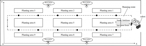
Figure 1 illustrates the scene of Wi-Fi positioning for material transport in a typical greenhouse. The greenhouse is 60m in length and 10m in width, for most greenhouses varies from 400 to 1,000m2 in size. It can be seen that the greenhouse is divided by 2m-wide roads into several planting areas. The vehicle can drive freely through these roads. Four BS nodes are located on the edges of the greenhouse, such that the Wi-Fi signal can cover the entire scene.
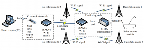
Based on the scene in Figure 1, the structure of our Wi-Fi positioning system was designed as shown in Figure 2. Our system mainly consists of four BS nodes, one communication node and a positioning node. The BS nodes are responsible for transmitting the Wi-Fi signal, the communication node is responsible for data exchange, and the positioning node is responsible for data collection and computation. The functions of these nodes need to be optimized through the balanced design of circuits, autonomous control module and positioning module.
Figure 1. The scene of Wi-Fi positioning for material transport in a typical greenhouse
Figure 2. The structure of our Wi-Fi positioning system
2.2 Circuit design
2.2.1 Selection and deployment of BS nodes
The BS nodes mainly transmit the Wi-Fi signal across the entire area of the greenhouse. These nodes should be selected based on the relationship between the transmission power Pt and transmission distance d of the Wi-Fi device. Obviously, the power of the Wi-Fi signal is negatively correlated with the transmission distance [20]. The RSSI at transmission distance d can be computed by:
$R S S I_{d}=R S S I_{d_{0}}-10 \times n \times \lg \left(\frac{d}{d_{0}}\right)$ (1)
where, n is the path-dependent power loss index; RSSId0 is the RSSI at transmission distance d0.
The transmission power of the Wi-Fi device Pt (dBm) can be expressed as:
$P_{t}=P_{r}-G_{t}+G_{r}+B_{t}+M+L_{d}$ (2)
where, Pr is the receiving power (dBm); Gt and Gr are the gains of the transmitting and receiving antennas (dBi), respectively; Bt is the loss of the combined, feedline or waveguide (dB); M is the fading margin (dB); Ld is the free space loss (dB).
Then, the free space transmission loss Ld (dB) of the Wi-Fi signal can be described as:
$L_d (dB)=32.44+20 lgd (km)+20 lgf (MHz)$ (3)
where, d is the transmission distance; f is the operating frequency. Thus, the free space transmission loss is only associated with the transmission distance and the operating frequency.
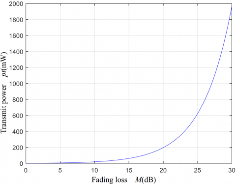
If a BS node is installed in each corner of the 60m×10m greenhouse, the signal range, target transmission distance, operating frequency, receiving power, transmitting antenna gain, receiving antenna gain and the loss of the combined, feedline or waveguide of each BS can be obtained as $\sqrt[2]{60^{2}+10^{2}}=60.8(m)$, $d=60(m)=0.06(km)$, $f=2.5(GHz)=2500(MHz)$, $P_r=-70(dB)$, $G_t=10(dBi)$, $G_r=3(dBi)$, and $B_t=10(dB)$, respectively. Substituting these results to formula (3), the free space transmission loss can be derived as $L_d=75.96(dB)$. Then, the relationship between transmission power and fading loss can be obtained by substituting the calculated values to formula (2). Through MATLAB simulation with the transmission distance of 60m (i.e. the length of the typical greenhouse), the relationship can be illustrated by the curve in Figure 3 below.
Figure 3. Relationship between the transmission power and the fading loss
In greenhouse environment, the fading loss generally falls between 20 and 25dB. Hence, the transmission power of BS nodes should range between 400 and 600mW, i.e. 26.02dBm and 27.78dBm. On this basis, LF-OAP50 outdoor high-power BS (Lafalink, China) was selected for the BS nodes in our system. The transmission power and receiving sensitivity of the BS are 27dBm (500mW) and -72dB, respectively.
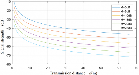
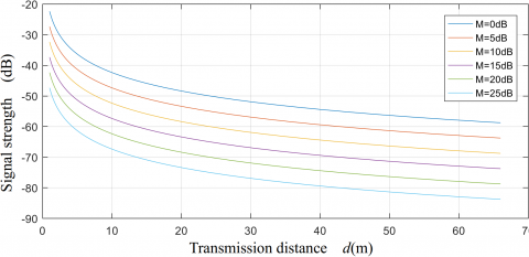
Next, the BS nodes were positioned based on the relationship between the RSSI of Wi-Fi signal and transmission distance. For the LF-OAP50 outdoor high-power BS, the said relationship was simulated on MATLAB in greenhouse environments with different fading losses M (M=0-25dB). The simulation results (Figure 4) show that the RSSI has a negative correlation with the transmission distance. Within the transmission distance of 60m, the peak RSSI of the BS was -71dB, greater than the receiving sensitivity (-72dB). Hence, the Wi-Fi signal will not be distorted during the transmission over 60m. In other words, the LF-OAP50 outdoor high-power BS meets the design requirements of our system.
Figure 4. The relationship between RSSI and transmission distance at the transmission power of 500mW
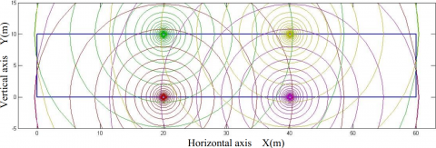
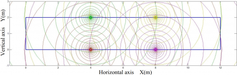
Finally, the four BS nodes were deployed to maximize the distortion-free coverage and the availability of signal range (i.e. the ratio of BS signal range to the circumference). Three BS nodes were arranged for positioning, and the other for position correction. Under this arrangement, the Wi-Fi signal from each BS can be received at any position, and the RSSIs of the signals from the three BSs are unequal at any position. The placement and signal attenuation ranges of the four BSs are displayed in Figure 5. The signal attenuation ranges were obtained through MATLAB simulation. It can be seen that, under the BS arrangement, the entire greenhouse was covered by Wi-Fi signals and the signals were utilized efficiently. Hence, the BS arrangement was adopted for our system.
Figure 5. Signal attenuation ranges of the four BSs
2.2.2 Circuit design of positioning node
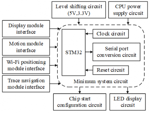
The positioning node serves to collect and process the RSSIs of the Wi-Fi signals from the BS nodes, and transmit the resulting positions via the Wi-Fi module. As shown in Figure 6, the circuit of this node is composed of a Wi-Fi module and an STM32 minimum system. The two systems are connected via a serial port. The STM32, including a clock circuit, a reset circuit and a serial port conversion circuit, collect the RSSI of the Wi-Fi signal from each BS and calculate the BS position. Based on the calculated BSs, the STM32 controls the navigation module and the motion module via the serial port, and then regulates the speed and direction of the unmanned vehicle.
Figure 6. The circuit design of positioning node
2.2.3 Circuit design of communication node
The communication node aims to receive the positions transmitted by the node at the COM port of the host computer, and displays the positions on the host computer via the serial port. As shown in Figure 7, the circuit of communication node mainly includes a Wi-Fi module, an LED display circuit of working status, a reset circuit, a serial port conversion circuit and a power conversion & switching (PCS) circuit. The positioning node communicates with other nodes using Wi-Fi signals. Specifically, the communication node is an ESP8266 chip; the serial port conversion circuit links up the chip with the host computer; the LED indicates whether the positions are received by the chip; the reset circuit initializes the chip; the PCS circuit provides stable power to the chip.
Figure 7. The circuit design of communication node
2.3 Positioning algorithm
Based on RSSI ranging and the MLE, an efficient and low-cost positioning algorithm was designed for the unmanned vehicle. Firstly, the RSSIs at the positioning node were measured. Then, the corresponding transmission distances were calculated by the signal attenuation model, which is a curve inferred from multiple measurements and the relationship between the transmission distance and RSSI of the Wi-Fi signal. The transmission distance d can be calculated by:
$d=10^{\left(\frac{R S S I_{d}-R S S I_{d_{0}}}{10 \times n}\right)}$ (4)
The position of the positioning node was derived from the coordinates of each BS node and the transmission distance from each BS node to the positioning node. The derivation utilizes the MLE, a triangulation method for positioning.
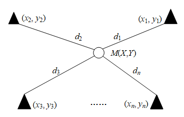
Figure 8. The principle of the MLE
As shown in Figure 8, there are n BS nodes with known coordinates: $\left(x_{1}, y_{1}\right),\left(x_{2}, y_{2}\right),\left(x_{3}, y_{3}\right) \ldots\left(x_{n}, y_{n}\right)$. The distances between each BS node and the positioning node M are denoted as $d_{1}, d_{2}, d_{3}$ and $d_{n}$, respectively. Then, the following set of equations can be established:
$\left\{\begin{array}{l}\left(x-x_{1}\right)^{2}+\left(y-y_{1}\right)^{2}=d_{1}^{2} \\ \left(x-x_{2}\right)^{2}+\left(y-y_{2}\right)^{2}=d_{2}^{2} \\ \vdots \\ \left(x-x_{n}\right)^{2}+\left(y-y_{n}\right)^{2}=d_{n}^{2}\end{array}\right.$ (5)
Subtracting the first the $n-1$ equations from the last $n^{t h}$ equations, we have:
$\left\{\begin{array}{c}x_{1}^{2}-x_{n}^{2}-2\left(x_{1}-x_{n}\right) x+y_{1}^{2}-y_{n}^{2}-2\left(y_{1}-y_{n}\right) y=d_{1}^{2}-d_{n}^{2} \\ x_{2}^{2}-x_{n}^{2}-2\left(x_{2}-x_{n}\right) x+y_{2}^{2}-y_{n}^{2}-2\left(y_{2}-y_{n}\right) y=d_{2}^{2}-d_{n}^{2} \\ \vdots \\ x_{n-1}^{2}-x_{n}^{2}-2\left(x_{n-1}-x_{n}\right) x+y_{n-1}^{2}-y_{n}^{2}-2\left(y_{n-1}-y_{n}\right) y=d_{n-1}^{2}-d_{n}^{2}\end{array}\right.$ (6)
Then, the position of the positioning node can be obtained by:
$\boldsymbol{X}=\left(\boldsymbol{A}^{\mathrm{T}} \boldsymbol{A}\right)^{-1} \boldsymbol{A}^{\mathrm{T}} \boldsymbol{B}$ (7)
where,
$A=\left(\begin{array}{cc}2\left(x_{1}-x_{n}\right) & 2\left(y_{1}-y_{n}\right) \\ \vdots & \vdots \\ 2\left(x_{n-1}-x_{n}\right) & 2\left(y_{n-1}-y_{n}\right)\end{array}\right)$
$\boldsymbol{B}=\left(\begin{array}{c}x_{1}^{2}-x_{n}^{2}+y_{1}^{2}-y_{n}^{2}+d_{n}^{2}-d_{1}^{2} \\ \vdots \\ x_{n-1}^{2}-x_{n}^{2}+y_{n-1}^{2}-y_{n}^{2}+d_{n-1}^{2}-d_{1}^{2}\end{array}\right), \boldsymbol{X}=\left(\begin{array}{l}x \\ y\end{array}\right)$ (8)
In the light of our system design, n=4 was substituted into formulas (7) and (8) to obtain the coordinates of the positioning node. Let $A P_{1}\left(2 x_{0}, 0\right), A P_{2}\left(2 x_{0}, y_{0}\right), A P_{3}\left(4 x_{0}, y_{0}\right) and A P_{4}\left(4 x_{0}, 0\right)$ be the coordinates of the four BS nodes, respectively. Formulas (7) can be simplified as:
$x=\frac{36 x_{0}^{2}+2 d_{1}^{2}-d_{2}^{2}+d_{3}^{2}-2 d_{4}^{2}}{12 x_{0}}$ (9)
$y=\frac{3 y_{0}^{2}-2 d_{1}^{2}+d_{2}^{2}+2 d_{3}^{2}-d_{4}^{2}}{6 y_{0}}$ (10)
2.4 Programs of our system
Our system involves a Wi-Fi module drive program, a data acquisition program, a positioning program, and a communication protocol program. The workflow of our system is as follows: First, the operating mode is set for each BS node, which then transmits a Wi-Fi signal of a certain frequency. Next, the communication node and positioning node are configured. After that, the positioning node collects Wi-Fi signals from the BS nodes. Based on the RSSIs of the received signals, the STM32 calculates the position of each BS node, and sends the positions to the communication node. Then, the communication node uploads the BS node positions to the host computer via the serial port, and derives the coordinates of the positioning node.
The main function of each BS node is to provide the RSSI that reflects the transmission distance. Once powered, each BS node is deployed at the position of the right coordinates. On the same plane, the positioning node can be located based on the coordinates of the four BS nodes.
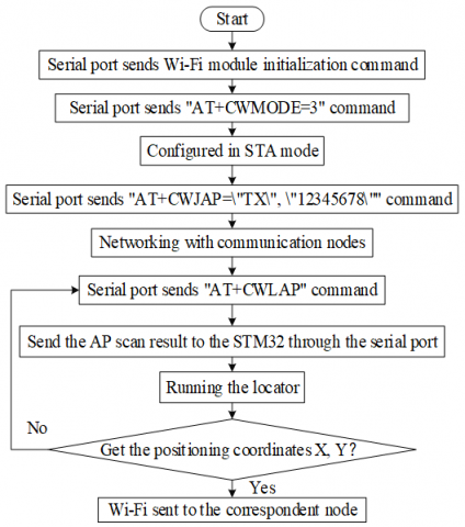
The positioning node has a Wi-Fi module and an STM32F103 microcontroller. The node measures the RSSI from each BS node, derives the position of each BS, and exchanges data with the communication node. The STM32 uses attention commands to configure and communicate with the Wi-Fi module. Once initialized, the Wi-Fi module (Figure 9) of the positioning node is configured at the station mode. Then, the RSSI of the peripheral access point is scanned continuously. The scanned data are sorted and returned to STM32 via the serial port. To prevent the positioning from being affected by signal fluctuations, the median filtering method is employed to process the data. Based on the processed data, the BS node positions are calculated and reported to the communication node.
Figure 9. The workflow of the Wi-Fi module in the positioning node
The communication node acts as a data transfer station between the positioning node and the host computer. The main functions include uploading the positions and forwarding the control commands from the host computer. The programs of this node include networking command program and communication program.
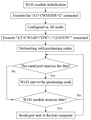
As shown in Figure 10, the communication node is configured after all nodes are initialized and the positioning system enters normal operation. The working mode, positioning node and serial baud rate are configured. After the configuration, the communication node enters the message detection mode to judge whether the Wi-Fi module has received data. If yes, the serial port will upload the received data to the host computer. Then, the positions will be displayed on the display interface.
Figure 10. The workflow of the Wi-Fi module of the communication node
3.1 Simulation
During the simulation, the BS nodes were emulated by the ESP8266 chip, a component of positioning and communication nodes. The chip realizes virtually all the functions of the Wi-Fi network. It can work independently or work together with a microcontroller. All the four BS nodes were set to the SoftAP mode.
Based on the parameters of formulas (2) and (3) and the ESP8266 chip, a MATLAB simulation was performed to verify the relationship between the RSSI of the Wi-Fi signal from each BS node and the transmission distance in different greenhouse environments, i.e. at different fading losses M. According to the simulated relationship in Figure 11, when the M increased from 0 to 25dB, the RSSI of ESP8266 chip, whose receiving sensitivity is -75dB, attenuated to -72dB at the most in the range of 20m. Hence, the chip can maintain a good RSSI in the range of 20m. In the range of 60m, the RSSI attenuation exceeded -75dB, failing to meet the simulation requirements. It can be seen that the signal attenuation of the chip within 20m is basically similar to that of the LF-OA50 within 60m.
In the light of the similarity, an open concrete field of 12m´2m, which is a reduced scale of the 60m´10m greenhouse, was selected for simulation. The remote location of the field eliminates the interference from other Wi-Fi signals, ensuring the simulation accuracy. The simulation results in Figure 12 confirm the feasibility and applicability of the arrangement of the four BSs nodes.
Figure 11. The simulated relationship between the RSSI and transmission distance at the transmission power of 100mW
Figure 12. The simulated signal attenuation ranges of the four BSs
3.2 Ranging experiment
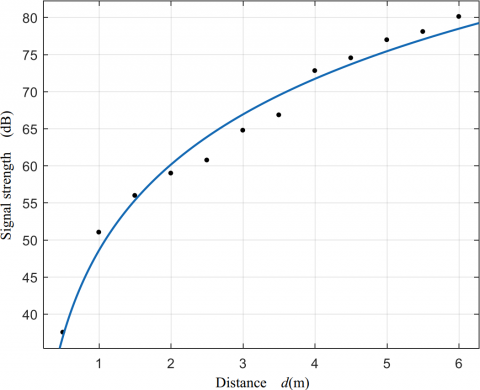
The propagation of the Wi-Fi signal is affected by various factors. Thus, the parameters of the Wi-Fi signal attenuation model may vary substantially with the application environments. Hence, a ranging experiment was carried out to disclose the exact relationship between the RSSI and transmission distance. As mentioned before, each BS node was emulated by the ESP8266 chip, and the 12m´2m open concrete field was used for the experiment. During the experiment, the RSSI at each node was computed by averaging the results of five measurements, and used to fit the signal attenuation model for the current positioning environment. The parameters of the model were corrected before the experiment. According to the experimental results (Table 1), the most suitable attenuation curve was fitted in MATLAB (Figure 13).
Based on Table 1 and Figure 13, the RSSI at the transmitter-receiver distance of 1m A and the attenuation coefficient n were respectively computed as 51 and 3.32. The A and n values were substituted into formula (1) to derive the relationship between the RSSI and transmission distance:
$R S S I=\log d \times 33.2+51$ (11)
Table 1. The results of the ranging experiment
|
Distance (m) |
0.5 |
1 |
1.5 |
2 |
2.5 |
3 |
|
RSSI (dB) |
37.52 |
51.01 |
55.96 |
58.97 |
60.73 |
64.75 |
|
Distance (m) |
3.5 |
4 |
4.5 |
5 |
5.5 |
6 |
|
RSSI (dB) |
66.82 |
72.79 |
74.51 |
76.95 |
78.06 |
80.09 |
Figure 13. The attenuation curve
3.3 Positioning system experiment
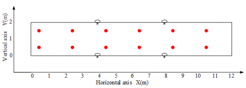
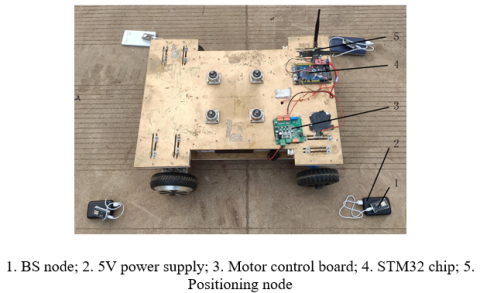
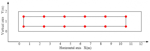
To verify the effectiveness of our positioning system, four BS nodes W1-W4 were fixed on the 12m´2m open concrete field (Figure 14). Twelve points (red asterisks) were selected for reference. In addition, a 2D coordinate system was established with the origin at the apex of the lower left corner of the field. The coordinates of W1-W4 are (4, 0), (4, 2), (8, 2) and (8, 0), respectively. The communication node was connected to the host computer, and the positioning node was linked up to the STM32 chip. Under this environment, the proposed system was applied to position the unmanned vehicle that transports materials to the warehouse. As shown in Figure 15, the vehicle is 650mm-long and 400mm-wide, and 300mm in wheel tread.
Figure 14. The experimental environment
Figure 15. The unmanned vehicle
Once the reset key of the positioning node was pressed, it only took a few seconds for the serial port debugging interface of the host computer to receive the position information from the positioning node. Then, the unmanned vehicle moved to every reference point. The position at each reference point was computed by averaging three repeated measurements. The positioning results are listed in Table 2.
Based on the positioning results, the authors plotted an expected route map (Figure 16) and a simulated route map (Figure 17). The experimental results show that our positioning system can function normally: the positioning node positioned the vehicle accurately based on the collected position data, laying the basis for material transport in the typical greenhouse. The 43.00cm deviation from the actual position indicates that the positioning results of our system are slightly poorer than the ideal results. Through data analysis, the error is identified as the large fluctuations of the RSSI at a fixed point, which depend on the positioned coordinates.
Table 2. The positioning results
|
Serial number |
Actual coordinates (X/m, Y/m) |
Positioned coordinates (X/m, Y/m) |
Deviation (cm) |
|
1 |
(0.5,0.5) |
(0.37,0.80) |
32.00 |
|
2 |
(0.5,1.5) |
(0.85,1.31) |
39.00 |
|
3 |
(2.5,0.5) |
(2.15,0.74) |
42.00 |
|
4 |
(2.5,1.5) |
(2.22,1.75) |
37.00 |
|
5 |
(4.5,0.5) |
(4.09,0.76) |
48.00 |
|
6 |
(4.5,1.5) |
(4.21,1.71) |
35.00 |
|
7 |
(6.5,0.5) |
(6.06,0.73) |
49.00 |
|
8 |
(6.5,1.5) |
(6.15,1.38) |
37.00 |
|
9 |
(8.5,0.5) |
(7.99,0.55) |
51.00 |
|
10 |
(8.5,1.5) |
(7.93,1.62) |
57.00 |
|
11 |
(10.5,0.5) |
(11.02,0.70) |
55.00 |
|
12 |
(10.5,1.5) |
(10.86,1.60) |
37.00 |
Figure 16. The expected route map
Figure 17. The simulated route map
3.4 Vehicle operation optimization
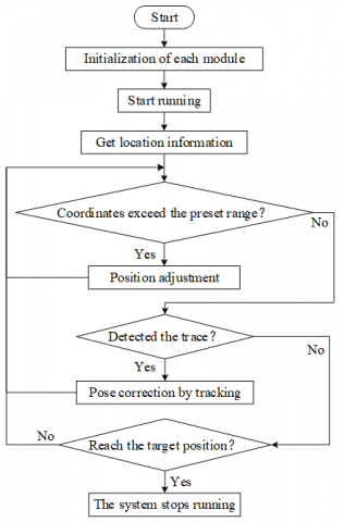
The system design was further improved to reduce the positioning error, such that the vehicle can move more accurately in actual greenhouses. Grayscale sensors with tracking function and lines were arranged on the ground of the greenhouse to improve the effectiveness of our system. Figure 18 presents the improved circuit structure, and Figure 19 explains the workflow of the improved system.
Figure 18. Circuit structure of optimized positioning node
Figure 19. Chart of improved workflow
According to the positioning results of the previous experiment, the deviation on the Y-axis was 43.00cm within the range of 1m on the X-axis. Therefore, the distance between every two reference points on the X-axis was divided into 5 segments by an interval of 40cm. Each division point was marked with a 20cm-long cross mark. The other settings remained unchanged, including the BS positions, number and positions of reference points, and the coordinate system. In addition, eight grayscale sensors were installed in the front of the vehicle, and the line-tracking program was embedded into the improved positioning system.
Under the above environment (Figure 20), the improved positioning system was applied to guide the unmanned vehicle in material transport. During normal operation, the vehicle relies on the Wi-Fi for positioning; if it encounters a cross mark, the vehicle moves along a straight line and corrects its posture by grayscale sensors. For each node, the coordinates of three reference points were collected, and the distances between the node and the BSs were measured and averaged. The results of the improved positioning system are listed in Table 3. Based on the results, the authors plotted a simulated route map (Figure 21).
Table 3. The improved positioning results
|
Serial number |
Actual coordinates (X/m, Y/m) |
Positioned coordinates (X/m, Y/m) |
Deviation (cm) |
|
1 |
(0.5,0.5) |
(0.5,0.55) |
5.00 |
|
2 |
(0.5,1.5) |
(0.5,1.59) |
9.00 |
|
3 |
(2.5,0.5) |
(2.5,0.57) |
7.00 |
|
4 |
(2.5,1.5) |
(2.5,1.56) |
6.00 |
|
5 |
(4.5,0.5) |
(4.5,0.59) |
9.00 |
|
6 |
(4.5,1.5) |
(4.5,1.45) |
5.00 |
|
7 |
(6.5,0.5) |
(6.5,0.57) |
7.00 |
|
8 |
(6.5,1.5) |
(6.5,1.55) |
5.00 |
|
9 |
(8.5,0.5) |
(8.5,0.56) |
6.00 |
|
10 |
(8.5,1.5) |
(8.5,1.54) |
4.00 |
|
11 |
(10.5,0.5) |
(10.5,0.57) |
7.00 |
|
12 |
(10.5,1.5) |
(10.5,1.59) |
9.00 |
Figure 20. The experimental environment
Figure 21. The improved simulated route map
The experimental results show that the mean deviation of the improved positioning system was 6.58cm in the experimental environment, thanks to the posture correction based on grayscale sensors. The improved system can fulfil the demand for material transport in greenhouse facilities: the farmers will work less laboriously and more efficiently due to the highly accurate positioning.
This paper designs a Wi-Fi positioning system for material transport in greenhouses. In the Wi-Fi coverage, the positioning algorithm of the positioning node was created based on RSSI ranging and the MLE. Through simulation and experiments, it is proved that the proposed system can locate the positioning node and report the results to the host computer. The accuracy of the system was further improved by grayscale sensors, meeting more challenging demands during material transport in greenhouses.
There are multiple advantages of the proposed positioning system: (1) The overall performance is superior than that of other positioning systems (e.g. Bluetooth positioning and ultrasonic positions), facing the wide coverage and stable attenuation of the Wi-Fi signal in the greenhouse; (2) The selected BS nodes, positioning node and communication node are cheap, reducing the total cost of the system; (3) Due to its small node size, the system can be easily expanded and optimized to suit new greenhouse environment.
In the future research, crop sheltering will be taken into account, and the RSSI fingerprint database and clustering algorithm will be combined to create an offline map to match the online positioning results.
This research has received support from the Shaanxi Key Research and Development Program of China (2019NY-171, 2019ZDLNY02-04, 2018TSCXL-NY-05-04), And Innovative Training Program for College Students of Northwest A&F University (No. 1201810712046). The authors are also gratefully to the reviewers for their helpful comments and recommendations, which make the presentation better.
[1] Ghoulem, M., El Moueddeb, K., Nehdi, E., Boukhanouf, R., Calautit, J.K. (2019). Greenhouse design and cooling technologies for sustainable food cultivation in hot climates: Review of current practice and future status. Biosystems Engineering, 183: 121-150. https://doi.org/10.1016/j.biosystemseng.2019.04.016
[2] Xu, P., Jia, C., Li, Y., Sun, Q., Liu, R. (2015). Developing an enhanced short-range railroad track condition prediction model for optimal maintenance scheduling. Mathematical Problems in Engineering, 2015: 796171. https://doi.org/10.1155/2015/796171
[3] Mendes, A.S., Villarrubia, G., Caridad, J., Daniel, H., De Paz, J.F. (2019). Automatic wireless mapping and tracking system for indoor location. Neurocomputing, 338: 372-380. https://doi.org/10.1016/j.neucom.2018.07.084
[4] Zhang, Y., Zhang, G., Du, W., Wang, J., Ali, E., Sun, S. (2015). An optimization method for shopfloor material handling based on real-time and multi-source manufacturing data. International Journal of Production Economics, 165: 282-292. https://doi.org/10.1016/j.ijpe.2014.12.029
[5] Morales, J.A., Akopian, D., Agaian, S. (2014). Faulty measurements impact on wireless local area network positioning performance. IET Radar, Sonar & Navigation, 9(5): 501-508. https://doi.org/10.1049/iet-rsn.2014.0108
[6] He, S., Chan, S.H.G. (2015). Wi-Fi fingerprint-based indoor positioning: Recent advances and comparisons. IEEE Communications Surveys & Tutorials, 18(1): 466-490. https://doi.org/10.1109/COMST.2015.2464084
[7] Luo, X., Wang, H., Yan, S., Liu, J., Zhong, Y., Lan, R. (2018). Ultrasonic localization method based on receiver array optimization schemes. International Journal of Distributed Sensor Networks, 14(11): 1550147718812017. https://doi.org/10.1177/1550147718812017
[8] Yasir, M., Ho, S.W., Vellambi, B.N. (2015). Indoor position tracking using multiple optical receivers. Journal of Lightwave Technology, 34(4): 1166-1176. https://doi.org/10.1109/JLT.2015.2507182
[9] Guan, W., Chen, X., Huang, M., Liu, Z., Wu, Y., Chen, Y. (2018). High-speed robust dynamic positioning and tracking method based on visual visible light communication using optical flow detection and Bayesian forecast. IEEE Photonics Journal, 10(3): 1-22. https://doi.org/10.1109/JPHOT.2018.2841979
[10] Huang, B., Liu, J., Sun, W., Yang, F. (2019). A Robust indoor positioning method based on Bluetooth Low energy with Separate channel information. Sensors, 19(16): 3487. https://doi.org/10.3390/s19163487
[11] Qureshi, U.M., Umair, Z., Hancke, G.P. (2019). Evaluating the implications of varying Bluetooth low energy (BLE) transmission power levels on wireless indoor localization accuracy and precision. Sensors, 19(15): 3282. https://doi.org/10.3390/s19153282
[12] Son, Y., Kim, S., Byeon, S., Choi, S. (2018). Symbol Timing Synchronization for Uplink Multi-User Transmission in IEEE 802.11 ax WLAN. IEEE Access, 6: 72962-72977. https://doi.org/10.1109/ACCESS.2018.2881980
[13] Lee, S., Kim, J., & Moon, N. (2019). Random forest and WiFi fingerprint-based indoor location recognition system using smart watch. Human-centric Computing and Information Sciences, 9(1): 6. https://doi.org/10.1186/s13673-019-0168-7
[14] Molebny, V., McManamon, P.F., Steinvall, O., Kobayashi, T., Chen, W. (2016). Laser radar: historical prospective-from the East to the West. Optical Engineering, 56(3): 031220. https://doi.org/10.1117/1.OE.56.3.031220
[15] Laitinen, E., Lohan, E.S. (2016). On the choice of access point selection criterion and other position estimation characteristics for WLAN-based indoor positioning. Sensors, 16(5): 737. https://doi.org/10.3390/s16050737
[16] Ma, Z., Wu, B., Poslad, S. (2019). A WiFi RSSI ranking fingerprint positioning system and its application to indoor activities of daily living recognition. International Journal of Distributed Sensor Networks, 15(4): 1550147719837916. https://doi.org/10.1177/1550147719837916
[17] Sadowski, S., Spachos, P. (2018). Rssi-based indoor localization with the internet of things. IEEE Access, 6: 30149-30161. https://doi.org/10.1109/ACCESS.2018.2843325
[18] Gómez-Tornero, J.L., Cañete-Rebenaque, D., López-Pastor, J.A., Martínez-Sala, A.S. (2018). Hybrid analog-digital processing system for amplitude-monopulse RSSI-based MIMO WiFi direction-of-arrival estimation. IEEE Journal of Selected Topics in Signal Processing, 12(3): 529-540. https://doi.org/10.1109/JSTSP.2018.2827701
[19] Xue, W., Qiu, W., Hua, X., Yu, K. (2017). Improved Wi-Fi RSSI measurement for indoor localization. IEEE Sensors Journal, 17(7): 2224-2230. https://doi.org/10.1109/JSEN.2017.2660522
[20] Svečko, J., Malajner, M., Gleich, D. (2015). Distance estimation using RSSI and particle filter. ISA Transactions, 55: 275-285. https://doi.org/10.1016/j.isatra.2014.10.003