Rouan Serik Habib* | Bounif Abdelhamid | Bouzit Mohamed | Ahmed Amine Larbi
OPEN ACCESS
This paper mainly numerically simulates the reactive flow of a hydrogen flame diluted with nitrogen. The behavior of this flame was simulated by two turbulence models: the standard k-epsilon (k-ε) model and the Reynolds stress model (RSM). The combustion process was modelled by the probability density function (PDF), in association with the flamlete regime. For comparison, the authors measured the reactive flow of the said flame in a simple configuration under the simulation conditions. The measured results agree well with the simulation results: the RSM consistently outputted better results than the k-ε model in all flame zones. The research results are of great significance to the numerical visualization of turbulent gas flows.
reactive flow, flamelet regime, turbulence, combustion, numerical simulation
Hydrogen is one of the new clean energy alternatives for the future. It has the advantage of having a completely clean combustion, because its oxidation produces no greenhouse gas or other pollutant harmful to health. Studies of the combustion of hydrogen are therefore of considerable interest for scientific research in the industrial world.
In most energy systems Turbulence plays a predominant role in reactive flows. The study of turbulent reactive flows makes it possible to solve the characteristic equations resulting from fluid mechanics, thermodynamics and chemistry. Much research has focused on the influence of various aspects of turbulence models in understanding the physics of free and reactive flows:
Yilmaz et al. [1] validated H2/air combustion modeling results by comparing different models of turbulence. The impact of the performance of these models on the detailed characteristics of the combustion process was investigated by examining the internal and external temperature distribution of the combustion chamber; velocity, pressure, species and NOx profiles.
The main objective proposed in the paper Martin et al. [2] was a direct comparison with experimental results of a right and slightly rotating free-flow turbulent jet both experimentally and by means of CFD simulation with different turbulence models. It was shown that numerical simulation was a tool capable of accurately describing the type of flow being analyzed. Nevertheless, significant errors could be introduced if the incorrect turbulence model was applied. The direct and indirect effect of turbulence on combustion in the case of turbulent pre-mixed flames by a turbulent mixture has been investigated by Branley and Jones [3]. On the other hand, only the second order model for Reynolds tensions allows to taking into account the isothermal and reactive flow properties. A simulation of methanol flames and H2/CO bluff-body; is carried out by Roy and Sreedhara [4]. An attempt to establish the turbulence model accuracy in the calculation of the mixing fields; was performed for the prediction of chemical specie fractions and scalar field profiles.
In the work of Obula [5], an attempt was made to find the best mixture of fuel and air in supersonic engines (SCRAMJET). For this, a numerical analysis was carried out using ANSYS-FLUENT. Different turbulence models (k-ω and k-ε) were compared for a better understanding of the turbulence effect on the mixture of fuel and air. He also found the best turbulence model suited for this problem studied by combustion type SCRAMJET. Dutta et al. [6] have compared the influence of different turbulence models and selected a suitable turbulence model for a better numerical approach to flow phenomena in a tube vortex with an optimal calculation time. Sardasht et al. [7] have investigated the performance of several turbulence models for predicting the flux and heat transfer in forced convection of jets and air currents on a disc under various rotary stationary conditions. It was shown that if no RANS models develop well in all regions, the DDES-RKE model can capture all flows.
Liu et al. [8] have performed a numerical study of the separation corners of a highly loaded linear prescribed velocity distribution (PVD) compressor cascade using seven frequently used turbulence models for exact prediction of the separation flux of the corners. It was found that the standard k- ε model, the realizable k- ε model, the v2-f model, and the Reynolds RSM stress model can provide reasonable results for predicting the separation of three-dimensional corners. Thus the turbulence characteristics are discussed with concern anisotropy. Numerical validation to evaluate the influence of turbulence and combustion models was highlighted and conducted in a small-scale laboratory biomass furnace by Farokhi et al. [9]. Several chemical mechanisms (reduced and detailed chemical kinetics) were examined. Cui [10] has conducted on atmospheric turbulence modulation (MTF), and on the basis of approximation theory, in order to see the direct impact of what is called the introduced anisotropic factor; on the prediction of the turbulence with the turbulent constraints in particular with low Reynolds number. The effects of the interaction between turbulence and combustion for the diffusion flame were particular treated by Roekaerts et al. [11] using two approaches. Based on the evolution equation of the scalar-associated probability density (PDF) associated with a reduced chemical scheme (ILDM) and second a scalar PDF-based approach associated with a detailed chemical scheme.
Khan et al. [12] have undertaken CFD simulations using k-ε, RSM turbulence models. They apply their simulations to a column reactor at gas bubbles widely used in industry to highlight the implications of the simplification assumptions made in these turbulence models. Convective heat transfer and hydrodynamic characteristics of nano-fluids were studied by Larbi et al. [13] using ANSYS-FLUENT. They compared different turbulence models. The results showed that the anisotropy of the instantaneous velocity in the RSM model gave a higher turbulent kinetic energy. Popoola and Cao [14] have highlighted; the influence of turbulence models on the accuracy of the CFD analysis of a heat loop driven by a periodic motion. In order to improve the numerical models of the HMDHL, different models of turbulence were studied and compared with the experimental results to select the most appropriate turbulence modeling technique. A new integral validation technique is presented [15-17] to evaluate whether a turbulence model can correctly predict the flow physics in turn; the technique provides the information needed to improve the development of turbulence models.
The complexity of these equations makes analytical resolution limited to very simple cases. Direct resolution without a simplifying hypothesis requires immense computing power. The method used for the calculation is the RANS approach, which consists in averaging the equations of the phenomena [12]. The equations of mean quantities resulting from this approach reveal an unknown term which must be determined; it is the average reaction rate Z. Due to the strong nonlinearity of the reaction rates of the different species, its estimation is not direct and must be based on a phenomenological approach and therefore the equations governing such a phenomenon are:
2.1 Equation of continuity
$\frac{\partial \rho}{\partial \mathrm{t}}+\frac{\partial\left(\rho \mathrm{U}_{\mathrm{i}}\right)}{\partial \mathrm{x}_{\mathrm{i}}}=0$ (1)
2.2 Momentum equation
The equation of momentum for an incompressible and Newtonian fluid is given by:
$\frac{\partial \left( \rho {{u}_{i}} \right)}{\partial t}+\underbrace{\frac{\partial \left( \rho {{u}_{i}}{{u}_{j}} \right)}{\partial {{x}_{j}}}}_{Convective\text{ }transport}={{F}_{i}}-\underbrace{\frac{\partial p}{\partial {{x}_{i}}}}_{Pressure\text{ }forces}+\underbrace{\frac{\partial }{\partial {{x}_{j}}}\left[ \mu \left( \frac{\partial {{u}_{i}}}{\partial {{x}_{j}}}+\frac{\partial {{u}_{j}}}{\partial {{x}_{i}}} \right)-\frac{2}{3}\left( \frac{\partial {{u}_{i}}}{\partial {{x}_{j}}} \right){{\delta }_{_{ij}}} \right]}_{Viscosity\text{ }forces}+{{S}_{i}}^{u}$ (2)
2.3 Turbulence modeling
2.3.1 First order modeling
The RNG model was obtained from a mathematical technique called the Renormalization Group. The RNG technique leads to a differential equation [8]:
$\partial \left( \frac{\overline{{{\rho }^{2}}}k}{\sqrt{\varepsilon \mu }} \right)=1.72\frac{\widehat{\upsilon }}{\sqrt{{{\widehat{\upsilon }}^{3}}+99}}d\widehat{\upsilon } \\ and \\ \widehat{\upsilon }=\frac{\sigma }{\mu }\left( \mu +\frac{{{\mu }_{t}}}{\sigma } \right)=\sigma +\frac{{{\mu }_{t}}}{\mu }$ (3)
The energy equation
$\begin{align} & \frac{\partial }{\partial t}\left( \rho E \right)+\frac{\partial }{\partial {{x}_{i}}}\left( \rho {{u}_{i}}E \right)=\frac{\partial }{\partial {{x}_{i}}} \\ & \left[ {{k}_{eff}}\frac{\partial T}{\partial {{x}_{i}}}-\sum{{{h}_{i}}{{J}_{j}}+{{u}_{i}}{{\left( {{\tau }_{ij}} \right)}_{eff}}} \right]+{{S}_{h}} \\ \end{align}$ (4)
$J=-\left( \rho {{D}_{i;m}}+\frac{{{\mu }_{t}}}{S{{c}_{t}}} \right)\frac{\partial {{Y}_{i}}}{\partial {{x}_{i}}} \\ and \\ \frac{\partial \overline{\rho }k}{\partial t}+\frac{\partial \overline{\rho }k\widetilde{{{u}_{i}}}}{\partial {{x}_{i}}}=\frac{\partial }{\partial {{x}_{j}}}\left[ \left( \mu +\frac{{{\mu }_{t}}}{{{\sigma }_{k}}} \right)\frac{\partial k}{\partial {{x}_{j}}} \right]+{{G}_{k}}+{{G}_{b}}-\overline{\rho }\varepsilon ~$ (5)
2.3.2 Second-order modeling
The Reynolds stress equation is defined as follows:
$\frac{\partial}{\partial \mathrm{x}_{\mathrm{k}}}\left(\bar{\rho} \widetilde{\mathrm{U}}_{\mathrm{k}} \mathrm{u}_{\mathrm{i}} \mathrm{u}_{\mathrm{j}}\right)=\widetilde{\mathrm{P}}_{\mathrm{ij}}+\widetilde{\mathrm{D}}_{\mathrm{ij}}+\widetilde{\varphi}_{\mathrm{ij}}-\frac{2}{3} \delta_{\mathrm{ij}} \bar{\rho} \widetilde{\varepsilon}$(6)
This last equation is solved for: $\widetilde{u u}, \widetilde{v v}$ rt $\widetilde{u v}$ fluctuations $\widetilde{w w}$ w are assumed to be equal to the radial fluctuations $\widetilde{v v}[2].$ Terms of production are expressed by
$\tilde{P}_{v}=-\bar{\rho}\left(\underset{\mathbf{u}_{i} \mathcal{u}_{k}}{\sim} \frac{\partial \tilde{\mathbf{U}}_{j}}{\partial \mathbf{x}_{\mathrm{k}}}+\underset{\mathbf{u}_{i} \mathcal{u}_{k}}{\sim} \frac{\partial \tilde{\mathbf{U}}_{i}}{\partial \mathbf{x}_{\mathrm{k}}}\right)$(7)
These are exact terms that do not require any modeling. They play an important role in the representation of the various mechanisms of creation turbulent stresses. Term of diffusion is modeled as follows:
$\widetilde{\mathrm{D}}_{\mathrm{ij}}=\mathrm{C}_{\mathrm{S}} \frac{\partial}{\partial \mathrm{x}_{\mathrm{k}}}\left[\left(\bar{\rho} \frac{\widetilde{\mathrm{k}}}{\widetilde{\varepsilon}} \underset{\mathbf{u}_{k} \mathcal{u}_{l}}{\sim}+\bar{\rho} \mathrm{v} \delta_{\mathrm{kl}}\right) \frac{\partial}{\partial \mathrm{x}_{1}}\left(\underset{\mathbf{u}_{i} \mathcal{u}_{j}}{\sim}\right)\right]$ (8)
Pressure-strain correlation term
The modeling of this term is based on the Poisson equation linking the fluctuating pressure to the velocity field.
$\mathop{{\tilde{\varphi }}}_{ij}\text{ }=\text{ }\overline{\mathop{\text{p}}^{\text{''}}\text{ ( }\frac{\mathop{\partial \text{ u}}_{\text{i}}^{\text{''}}}{\mathop{\partial \text{ }x}_{j}}\text{ }+\text{ }\frac{\mathop{\partial \text{ u}}_{\text{j}}^{\text{''}}}{\mathop{\partial \text{ }x}_{i}}\text{ )}}\text{ }=\text{ }\mathop{{\tilde{\varphi }}}_{\text{ij}}^{\text{(1)}}\text{ }+\text{ }\mathop{{\tilde{\varphi }}}_{\text{ij}}^{\text{(2)}}$ (9)
The first term of Rotta et al. [6], which represents the tendency to return to isotropy, is first modeled as follows:
$\mathop{{\tilde{\varphi }}}_{\text{ij}}^{\text{(1)}}\text{ }=\text{ -}\mathop{\text{C}}_{\text{1}}\text{ }\bar{\rho }\text{ }\tilde{\varepsilon }\text{ ( }\frac{\overset{\tilde{\ }}{\mathop{\mathop{\text{u}}_{\text{i}}\mathop{u}_{j}}}\,}{{\tilde{k}}}\text{ - }\frac{\text{2}}{\text{3}}\text{ }\mathop{\delta }_{\text{ij}}\text{ ) }=\text{ - }\mathop{\text{C}}_{\text{1}}\text{ }\bar{\rho }\text{ }\tilde{\varepsilon }\text{ }\mathop{\text{a}}_{\text{ij}}$ (10)
The second term concerning the interaction between mean motion and turbulence, also known as the fast term, is modeled using the simpler model called the IP model (Isotropization of Production), defined by:
$\widetilde{\phi}_{i j}^{(2)}=-C_{2}\left(\widetilde{P}_{i j}-\frac{2}{3} \delta_{i j} \widetilde{P}_{k}\right)$(11)
$\widetilde{\mathrm{P}}_{\mathrm{k}}=\frac{1}{2} \widetilde{\mathrm{P}}_{\mathrm{kk}}=-\bar{\rho} \underset{\mathbf{u}_{i} \mathcal{u}_{k}}{\sim} \frac{\partial \widetilde{\mathrm{U}}_{\mathrm{i}}}{\partial \mathrm{x}_{\mathrm{k}}}$ is the average rate of kinetic energy production of turbulence. The Constants of the couple (C1, C2); is based on experiments [11]. The modeled dynamic dissipation equation is of the following form:
$\frac{\partial}{\partial \mathrm{x}_{\mathrm{k}}}\left(\bar{\rho} \widetilde{\mathrm{U}}_{\mathrm{k}} \widetilde{\varepsilon}\right)=\widetilde{\mathrm{D}}_{\mathrm{e}}+\bar{\rho} \frac{\widetilde{\varepsilon}^{2}}{\widetilde{\mathrm{k}}} \widetilde{\Psi}(\varepsilon)$ (12)
The term contains all the effects of production and destruction of dynamic dissipation. This term is modeled using the form proposed by Roekaerts et al. [11],
$\widetilde{\Psi}(\varepsilon)=\mathrm{C}_{\varepsilon 1} \frac{\widetilde{\mathrm{P}}_{\mathrm{k}}}{\widetilde{\rho} \widetilde{\varepsilon}}-\mathrm{C}_{\varepsilon 2}$(13)
The modeling of the diffusion term $\widetilde{D}_{\varepsilon}$ is given by the following relationship:
$\widetilde{\mathrm{D}}_{\varepsilon}=\mathrm{C}_{\varepsilon} \frac{\partial}{\partial \mathrm{x}_{\mathrm{k}}}\left[\bar{\rho} \frac{\widetilde{\mathrm{k}}}{\widetilde{\varepsilon}} \mathrm{u}_{\mathrm{k}}^{\sim} \mathrm{u}_{1} \frac{\partial}{\partial \mathrm{x}_{1}}(\widetilde{\varepsilon})\right]$ (14)
These transport equations are in a cylindro-polar coordinate system can be given by the following general parabolic form:
$\frac{\partial}{\partial \mathrm{x}}(\bar{\rho} \mathrm{U} \widetilde{\Phi})+\frac{1}{\mathrm{r}} \frac{\partial}{\partial \mathrm{r}}(\mathrm{r} \bar{\rho} \mathrm{V} \widetilde{\Phi})=\frac{1}{\mathrm{r}} \frac{\partial}{\partial \mathrm{r}}\left(\mathrm{r} \bar{\rho} \mathrm{D} \frac{\partial \widetilde{\Phi}}{\partial \mathrm{r}}\right)+\mathrm{S} \Phi$ (15)
$S_{\Phi}$ Defined here the source terms for each variant, and
$\widetilde{\mathrm{P}}=-\bar{\rho} \widetilde{\mathrm{uv}} \frac{\partial \widetilde{\mathrm{U}}}{\partial \mathrm{r}}$ (16)
2.4 Modeling of non-premixed combustion
The idea is to separate the mixing problem from that of the flame structure the flammelet model is more suitable for indirect simulation for this flow type.
Average mixture fraction and its variance
A simple description of the turbulent mixture is obtained from the two fields: the average mixture fraction, $\tilde{z}$ and its variance,$\underset{z^{\prime \prime 2}}{\sim}$.
$\frac{\partial}{\partial t}(\bar{\rho} \tilde{z})+\frac{\partial}{\partial \mathbf{x}_{i}}\left(\bar{\rho} \tilde{\mathfrak{u}}_{i} \widetilde{z} \right)=\frac{\partial}{\partial \mathbf{x}_{i}}\left(\bar{\rho} D_{t} \frac{\partial \tilde{z}}{\partial \mathbf{x}_{i}}\right)$ (17)
$\frac{\partial}{\partial t}(\bar{\rho} \tilde{z}) + \frac{\partial}{\partial \mathbf{x}_{i}}\left(\bar{\rho} \tilde{\mathbf{u}}_{i} \tilde{z} \right) = \frac{\partial}{\partial \mathbf{x}_{\mathrm{i}}}\left(\bar{\rho} \mathbf{D}_{\mathrm{t}} \frac{\partial \tilde{\mathbf{z}}}{\partial \mathbf{x}_{\mathrm{i}}}\right) \frac{\partial}{\partial t}\left(\bar{\rho} \frac{\partial}{\partial t}\left(\bar{\rho} z^{\prime \prime 2}\right) \right)+ \frac{\partial}{\partial \mathbf{x}_{i}}\left(\bar{\rho} \tilde{\mathbf{u}}_{i} \underset{z^{\prime \prime 2}}{\sim} \right) = \frac{\partial}{\partial \mathbf{x}_{i}}\left(\bar{\rho} \mathrm{D}_{\mathrm{tl}} \frac{\underset{z^{\prime \prime 2}}{\sim}}{\partial \mathrm{X}_{\mathrm{i}}}\right)+ \bar{\rho} \mathrm{D}_{t2} \frac{\partial \tilde{z}}{\partial \mathbf{x}_{\mathrm{i}}} \frac{\partial \tilde{z}}{\partial \mathbf{x}_{\mathrm{i}}} -c \bar{p} \frac{\varepsilon}{\mathrm{k}}^{\underset{z^{\prime \prime 2}}{\sim}}$(18)
2.5 Flamelet equations
Considering some simplifying assumptions, the Equations of flammelettes are written:
$\rho \text{ }\frac{\partial \text{ }\mathop{\text{Y}}_{\text{k}}\text{ }}{\partial \text{ }t}\text{ }=\text{ }\frac{\rho \text{ }\chi }{\mathop{2Le}_{\text{k}}}\text{ }\frac{\mathop{\partial }^{2}\text{ }\mathop{\text{Y}}_{\text{k}}}{\mathop{\partial \text{ z}}^{2}}$ (19)
$\rho \text{ }\frac{\partial \text{ T }}{\partial \text{ }t}\text{ }=\text{ }\frac{\rho \text{ }\chi }{2}\text{ }\frac{\mathop{\partial }^{2}\text{ T}}{\mathop{\partial \text{ z}}^{2}}\text{ }$ (20)
The solutions for the mean values are then written:
$\tilde{Y}_{k}=\int_{0}^{+\infty} \int_{0}^{1} Y_{k}(z, \chi) P(z, \chi) d z d \chi$(21)
$\tilde{\mathrm{T}}=\int_{0}^{+\infty} \int_{0}^{1} \mathrm{T}(\mathrm{z}, \chi) \mathrm{P}(\mathrm{z}, \chi) \mathrm{d} \mathrm{z} \mathrm{d} \chi$ (22)
And their computations require knowledge of the joint probability density function P (z, χ). The most common approximation for determining the probability density function is to consider z and χ as statistically independent variables [8]. It can be expressed as:
$P\text{ (z, }\chi \text{) }=\text{ P (z) }\text{. P (}\chi \text{)}$ (23)
P (z) is determined using the assumed PDF. In this method, the functional form of the probability density function is fixed in advance as a function of the first moments of the fraction mixture z (in general $\tilde{z}$ et $\underset{z^{\prime \prime 2}}{\sim}$. And calculated at each point from the values of these moments whose field and function P (z) are obtained by Eqns. (14) & (15) [9].
Simulation of hydrogen flame diluted with nitrogen (75% H2 / 25% N2) is carried out in a simple configuration.
Geometrical configuration:
The geometrical configuration considered in this work is a combustion chamber; formed with a horizontal tube of outer diameter equal to Ø 400 mm (air). The central tube brings the fuel is Ø 8mm in diameter; with a velocity of 42.3 m / s, which provides a fairly turbulent regime, with a Reynolds number of Re = 9,300). The combustion chamber has a length of 1.20 m. The peripheral flow is an upstream airflow of up to 0.3 m / s. This flow is weakly turbulent and its initial intensity is equal to 5%. The field of study rests in its entirety on the development zone (flame zone). The "Fluent" code was used to simulate the transport of this H2 / air reactive flow. For turbulence / combustion simulation choices; are defined as follows:
The chemistry-turbulence interaction was modeled with the stationary flammelet approach for a Lewis number (Le = 1) [3].
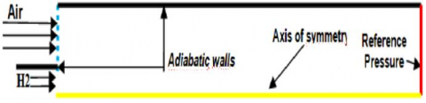
The boundary conditions used in a simulation are of several types. Their choice is a predominant element allowing the convergence or not of the computation, towards a logical solution. Indeed, an ill-exposed problem may well not admit a logical solution (divergence of the computation) or converge towards an illogical solution. The velocity input conditions are taken from experimental data [18]. An axisymmetric boundary is chosen on the jet axis, for the other boundaries, reference conditions of given reference pressure are chosen, as well as the conditions to the non-slip walls with adiabatic walls [11]. Table 1 presents the different values of the input conditions introduced exactly according to the experimental conditions [18]:
Table 1. Input conditions
|
Paramètres |
H2 (Jet) |
Air (Co-flow) |
|
Re |
9300 |
1200 |
|
D(mm) |
8 |
400 |
|
V(m/s) |
42.3 |
0.3 |
|
T(K) |
305 |
305 |
|
XH2 |
0,75 |
0.00 |
|
XO2 |
0,00 |
0,23 |
|
XN2 |
0,25 |
0,77 |
The different boundary conditions chosen in our simulation are illustrated in Figure 1:
Figure 1. Boundary conditions
Mesh Depency: in order to find an optimal mesh, different meshes have been tested. from 32,000 nodes, as shown in Figure 2 that the solution does not change significantly (<5%). We can therefore conclude that from a number of nodes, the solution does not change and becomes independent of the mesh.
Figure 2. Mesh choice
The mixing of the turbulent jet starts just at the outlet of the ejection nozzle; in this region the flow is very influenced by the inlet conditions, the same flow velocities and turbulent kinetic energy predicted by the two turbulence models are observed in Figure 3. Moreover, the magnitudes at the jet center (speed, turbulence. etc...) retain their initial value. It is only from (x/Dj = 20) that there is a difference of prediction between the two models. The axial evolutions of the temperature are represented in Figure 4.
Figure 3. Axial velocity evolution (U/Uj)
Figure 4. Axial temperature volution
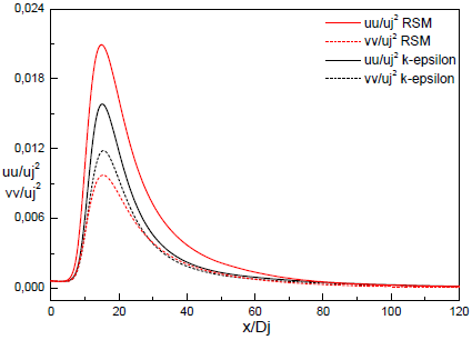
Figure 5. Turbulent contraints evolution
These evolutions present the same behavior as that of the experiment [17]. The maximum value reached by the RSM model is in the same amplitude and the same axial position as the experiment. The results obtained from the simulation are close to those of the experiment more particularly in the initial zone of the jet. However, this is not the case for the k-ε model which overestimates the results in the regions away from the ejection nozzle. For the temperature in Figure 4, it still appears that in the mixing zone of the reactants, the richness factor is high. This ensures a good mix of reagents and thus a higher efficiency of the burn rate. We can see from Figure 5, that the axial and radial turbulent stresses follow nearly similar evolutions although the intensities of (vv) are less strong than those of (uu).
Figure 6. Mixture fraction Z evolution
Figure 7. Mass fraction of H2 evolution
Figure 8. Mass fraction of N2 evolution
The RSM model predicts a real deviation between the maximal values of the axial (uu) and radial (vv) turbulent stresses as the k-ε model. Thus, the anisotropy of the flow is well detected by the RSM model. The axial evolution of the calculated average mixture fraction represented in Figure 6 is similar to that of the average mass fraction of H2. Both models of turbulence translate the same mixing rate with a slight convergence for RSM model towards the end part of the nozzle inlet compared to the experiment .The axial evolution of the average mass fractions of the majority H2 and N2 species shown in Figures (7-8); clearly shows a behavior of the two models of turbulence analogous to that of the experiment with a small overestimation of the experimental results in the regions close to the ejection nozzle.
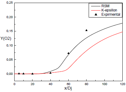
Figure 9. Mass fraction of O2 evolution
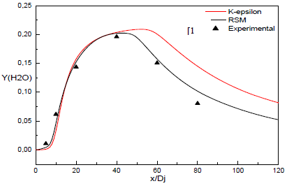
A good prediction of the experimental results by the two models is to be observed even in regions located at great distances from the ejection nozzle. Figures (9-10) show the axial evolution of the average mass fractions of the majority production species like (O2; H2O) ; Although good prediction is to be found for H2 two models of turbulence k-ε and RSM; but it may be noted that from x/D=50 the average mass fractions of O2/H2O, shows that the best prediction is used by the RSM model with a very good approach to experience. Also in regions located at great axial distances to the ejection nozzle, where other chemical phenomena are likely to be involved.
Figure 10. Mass Fraction of H2O evolution
This work is based on the flow visualization of an H2 diffusion flame, similar to that found in turbulent reactive jet measurements, using models (ke / RSM) as turbulence models. and the flamlete model for combustion modeling that seems to give good predictions in the equilibrium of chemical species. The results obtained show that predictions of flame zones based on the turbulence model (RSM) are generally slightly more credible than those obtained by the k-ε model, in particular those concerning the dynamic field of velocity and energy. Turbulent as well as its constraints. scalar fields for the majority species. In general, factors such as (diffusion effect, radiation, buoyancy, etc.) are neglected, turbulent kinetic energy measurements, the mixing fraction, the majority species and the temperature in the flame zones considered are reasonably consistent with the results. experimental with a better prediction advantage for the RSM Model of turbulence.
[1] Yilmaz, H., Cam, O., Tangoz, S., Yilmaz, I. (2017). Effect of different turbulence models on combustion and emission characteristics of hydrogen/air flames. International Journal of Hydrogen Energy, 42(40): 25744-25755. https://doi.org/10.1016/j.ijhydene.2017.04.080
[2] Miltner, M., Jordan, C., Harasek, M. (2015). CFD simulation of straight and slightly swirling turbulent free jets using different RANS-turbulence models. Applied Thermal Engineering, 89: 1117-1126. https://doi.org/10.1016/j.applthermaleng.2015.05.048
[3] Branley, N., Jones, W.P. (2001). Large eddy simulation of a turbulent non-premixed flame. Combustion and Flame, 127(1-2): 1914-1934. https://doi.org/10.1016/S0010-2180(01)00298-X
[4] Roy, R.N., Sreedhara, S. (2016). Modelling of methanol and H2/CO bluff-body flames using RANS based turbulence models with conditional moment closure model. Applied Thermal Engineering, 93: 561-570. https://doi.org/10.1016/j.applthermaleng.2015.09.073
[5] Kummitha, O.R. (2017). Numerical analysis of hydrogen fuel scramjet combustor with turbulence development inserts and with different turbulence models. International Journal of Hydrogen Energy, 42(9): 6360-6368. https://doi.org/10.1016/j.ijhydene.2016.10.137
[6] Dutta, T., Sinhamahapatra, K. P., Bandyopdhyay, S.S. (2010). Comparison of different turbulence models in predicting the temperature separation in a Ranque–Hilsch vortex tube. International Journal of Refrigeration, 33(4): 783-792. https://doi.org/10.1016/j.ijrefrig.2009.12.014
[7] Sardasht, M.T., Hosseini, R., Amani, E. (2017). An analysis of turbulence models for prediction of forced convection of air stream impingement on rotating disks at different angles. International Journal of Thermal Sciences, 118: 139-151. https://doi.org/10.1016/j.ijthermalsci.2017.04.021
[8] Liu, Y., Yan, H., Liu, Y., Lu, L., Li, Q. (2016). Numerical study of corner separation in a linear compressor cascade using various turbulence models. Chinese Journal of Aeronautics, 29(3): 639-652. https://doi.org/10.1016/j.cja.2016.04.013
[9] Farokhi, M., Birouk, M., Tabet, F. (2017). A computational study of a small-scale biomass burner: The influence of chemistry, turbulence and combustion sub-models. Energy Conversion and Management, 143: 203-217. https://doi.org/10.1016/j.enconman.2017.03.086
[10] Cui, L. (2018). Refractive-index fluctuations spectrum considering the general distribution of turbulence cells in moderate-to-strong anisotropic turbulence. Optik, 154: 473-484. doi.org/10.1016/j.ijleo.2017.10.082
[11] Roekaerts, D., Merci, B., Naud, B. (2006). Comparison of transported scalar PDF and velocity-scalar PDF approaches to ‘Delft flame III’. Comptes Rendus Mecanique, 334(8-9): 507-516. https://doi.org/10.1016/j.crme.2006.07.007
[12] Khan, Z., Bhusare, V.H., Joshi, J. B. (2017). Comparison of turbulence models for bubble column reactors. Chemical Engineering Science, 164: 34-52. https://doi.org/10.1016/j.ces.2017.01.023
[13] Larbi, A.A., Bounif, A., Senouci, M., Gökalp, I., Bouzit, M. (2018). RANS modelling of a lifted hydrogen flame using eulerian/lagrangian approaches with transported PDF method. Energy, 164: 1242-1256. https://doi.org/10.1016/j.energy.2018.08.073
[14] Popoola, O., Cao, Y. (2016). The influence of turbulence models on the accuracy of CFD analysis of a reciprocating mechanism driven heat loop. Case Studies in Thermal Engineering, 8: 277-290. https://doi.org/10.1016/j.csite.2016.08.009
[15] Larbi, A.A., Bounif, A., Bouzit, M. (2018). Comparisons of LPDF and MEPDF for lifted H-2/N-2 jet flame in a vitiated coflow. International Journal of Heat and Technology, 36(1): 133-140. https://doi.org/10.18280/ijht.360118
[16] Pond, I., Ebadi, A., Dubief, Y., White, C.M. (2017). An integral validation technique of RANS turbulence models. Computers & Fluids, 149: 150-159. https://doi.org/10.1016/j.compfluid.2017.02.016
[17] Larbi, A.A., Bounif, A., Bouzit, M. (2018). Modeling and numerical study of H2/N2 jet flame in vitiated co-flow using Eulerian PDF transport approach. Mechanics & Industry, 19(5): 504. https://doi.org/10.1051/meca/2018029
[18] Prucker, S., Meier, W., Stricker, W. (1994). A flat flame burner as calibration source for combustion research: Temperatures and species concentrations of premixed H2/air flames. Review of Scientific Instruments, 65(9): 2908-2911. https://doi.org/10.1063/1.1144637