Shunqing Ren* | Chunmei Dong | Xijun Chen | Changhong Wang
OPEN ACCESS
To optimize the systematic calibration of strapdown inertial navigation system (SINS), this paper derives a systematic calibration model according to the relationship between IMU’s errors and velocity errors output by navigation algorithm of IMU. Then, the advantages of horizontal three-axis turntable (3AT) where IMU errors are calibrated were utilized to decouple the mounting misalignments of the IMU, and an equal interval rotation test plan was designed to provide 16 rotation stimuli for the IMU. On the basis of it, the three sets of coupling relations of IMU’s mounting misalignments were decoupled, and the systematic calibration model was applied successfully in identifying 21 errors, including scale factor errors, biases and mounting misalignment. The simulation results show that, when the accelerometers and gyros in the IMU were at the accuracies of 10μg and 0.01°/h, respectively, the uncertainty of the accelerometer biases was 3.6mg and of the gyro’s biases was 0.004°/h. Finally, a 24h pure inertial navigation simulation was conducted in static positions. The attitude errors of systematic calibration are 6² in the x- and y-directions, and 2.2¢ in the z-direction, respectively, the maximum velocity error of systematic calibration was smaller than 0.3m/s. These results fully demonstrate the effectiveness of the systematic calibration method for the IMU calibrated on horizontal 3AT. This method suppresses the effects of turntable errors, and enhances the calibration accuracies of IMU.
SINS, systematic calibration, horizontal three-axis turntable (3AT), errors, gyro
The inertial navigation system (INS) is a completely self-contained navigation system that requires no external information. Therefore, the system possesses good concealment, stays immune to interference and supports all-weather operations [1-4]. The INS error mainly comes from the output errors of the inertial measurement unit (IMU). To minimize its impact on navigation accuracy, the output errors must be modelled and calibrated before use, and compensated during the utilization. The common calibration methods are classified into the separated and the systematic calibration method [5, 6].
The systematic calibration came into being in the 1980s, and has become the trend of calibration development. In systematic calibration, the output errors of the IMU, such as attitude error, velocity error and position error, are treated as observed quantities [7-10], and used to calibrate the parameters in the IMU error model [11-15], reducing the calibration dependence on the turntable’s accuracy. This method is a desirable way to carry out filed calibration, and a hotspot in relevant research [16].
Much research has conducted on the systematic calibration method. For instance, Lee and Sung [17] identified the scale factors and mounting misalignments of the accelerometers and the gyros, as well as the biases of gyros, using systematic calibration. In addition, Lee estimated the biases of gyro according to the additional control signals from closed-loop self-aligning system, and designed the corresponding calibration path. Considering three sets of rotational paths, Rogers [18] calibrated the IMU errors using the velocity error as observation in the navigation information. Savage [19] put forward two sets of rotation sequences, and compared the specific forces components before and after rotation, thereby calibrating the errors of accelerometer and gyro. Yang and Huang [20] established a systematic calibration model based on velocity error observation, and implemented progressive calibration of IMU errors: the scale factors and the biases of the gyros and the accelerometers were identified through systematic calibration, and then the mounting misalignments of the IMU were decoupled by separated calibration. Wu et al. [21] probed deeply into the reason for the coupling between the mounting misalignments of the IMU, and proposed a decoupling method to null gyro’s anti-symmetric matrix.
The traditional systematic calibration either relies on multi-positions excitation and angular rate excitation. However, the multi-position excitation only provides the input specific forces for calibrating accelerometer errors, while the angular rate excitation calibration only provides the input angular rate excitation and uses it for calibrating the gyro’s errors. The horizontal three-axis turntable (3AT), in which the outer axis is horizontal, can greatly simulate the IMU errors, making it easier to calibrate the errors. During the velocity calibration of gyro, the horizontal 3AT provides alternating input of specific forces to the accelerometer in three directions.
Considering the advantage of multi-position excitation using horizontal 3AT, this paper designs an equal interval rotation test plan to decouple the mounting misalignments of the IMU. Next, the author analyzed the relationship between the observables excited by the horizontal 3AT and the IMU errors. One the basis of it, he coupling between IMU’s mounting misalignments was eliminated, and 21 IMU errors were identified successfully, including scale factor, biases and mounting misalignments.
The output errors of strapdown inertial navigation system (SINS) can be described as:
$\delta {{\mathbf{f}}^{b}}=\delta {{\mathbf{M}}_{a}}{{\mathbf{f}}^{b}}+{{\mathbf{B}}_{a}}$ (1)
$\delta \mathbf{\omega }_{ib}^{b}=\delta {{\mathbf{M}}_{g}}\mathbf{\omega }_{ib}^{b}+{{\mathbf{B}}_{g}}$ (2)
where, ${{\mathbf{f}}^{b}}$ and $\mathbf{\omega }_{ib}^{b}$ are the inputs of the accelerometers and the gyro’s, respectively; $\delta {{\mathbf{M}}_{a}}=\left[ \begin{matrix} \Delta {{K}_{ax}} & 0 & 0 \\ {{M}_{ayx}} & \Delta {{K}_{ay}} & 0 \\ {{M}_{azx}} & {{M}_{azy}} & \Delta {{K}_{az}} \\\end{matrix} \right]$ (the diagonal and non-diagonal elements are the scale factors and the mounting misalignment of the accelerometers, respectively); $\delta {{\mathbf{M}}_{g}}=\left[ \begin{matrix} \Delta {{K}_{gx}} & {{M}_{gxy}} & {{M}_{gxz}} \\ {{M}_{gyx}} & \Delta {{K}_{gy}} & {{M}_{gyz}} \\ {{M}_{gzx}} & {{M}_{gzy}} & \Delta {{K}_{gz}} \\\end{matrix} \right]$ (the diagonal and non-diagonal elements are the scale factors and the mounting misalignments of the gyro’s, respectively); ${{\mathbf{B}}_{a}}={{\left[ \begin{matrix} {{B}_{ax}} & {{B}_{ay}} & {{B}_{az}} \\\end{matrix} \right]}^{\text{T}}}$ and ${{\mathbf{B}}_{g}}={{\left[ \begin{matrix} {{B}_{gx}} & {{B}_{gy}} & {{B}_{gz}} \\\end{matrix} \right]}^{\text{T}}}$ are the biases of the accelerometers and the gyro’s, respectively.
Taking the East-North-Up (ENU) as the navigation frame n, the velocity of the SINS can be expressed as:
$\mathbf{\dot{V}}_{en}^{n}={{\mathbf{f}}^{n}}-(2\mathbf{\omega }_{ie}^{n}+\mathbf{\omega }_{en}^{n})\times \mathbf{V}_{en}^{n}+{{\mathbf{g}}^{n}}$ (3)
The calibration experiment of the IMU consists of three steps, namely, alignment, rotation and stationary measurement. Let l be the aligned body frame, b be the rotated body frame, T1 be the rotation time, and t be the stationary measurement time.
From Eq. (3), the relationship between the IMU errors and velocity error can be obtained as [20]:
$\delta \mathbf{\dot{V}}_{en}^{n}={{\mathbf{Y}}_{2}}+{{\mathbf{Y}}_{1}}t$ (4)
where, ${{\mathbf{Y}}_{1}}=-\mathbf{C}_{b}^{n}(\mathbf{\tilde{\omega }}{{_{nb}^{b}}^{\times }})\mathbf{C}_{n}^{b}{{\mathbf{g}}^{n}}$, with $\mathbf{\tilde{\omega }}_{nb}^{b}$ is angular velocity of the b-frame relative to the n-frame in the stationary measurement time and can be regarded as constant approximately. Let ${{\mathbf{p}}^{\times }}$ be the anti-symmetric matrix of a random vector $\mathbf{p}$. ${{\mathbf{Y}}_{2}}$ can be described as [20]:
$\begin{align} & {{\mathbf{Y}}_{2}}=-\mathbf{C}_{b}^{n}\delta {{\mathbf{M}}_{a}}\mathbf{C}_{n}^{b}{{\mathbf{g}}^{n}}+\mathbf{C}_{b}^{n}{{\mathbf{B}}_{a}}+\left[ \begin{matrix} -{{\left[ \mathbf{C}_{l}^{n}\delta {{\mathbf{M}}_{a}}\mathbf{C}_{n}^{l}{{\mathbf{g}}^{n}}+\mathbf{C}_{l}^{n}{{\mathbf{B}}_{a}} \right]}_{\text{H}}} \\ 0 \\\end{matrix} \right]-\mathbf{C}_{l}^{n}\left\{ \frac{\sin a}{a}[\delta \mathbf{\sigma }\times ]+\frac{(1-\cos a)}{{{a}^{2}}}([\mathbf{\sigma }\times ][\delta \mathbf{\sigma }\times ]+[\delta \mathbf{\sigma }\times ][\mathbf{\sigma }\times ]) \right.+\text{ } \\ & \text{ }\left( \frac{(a\cos a-\sin a){{\mathbf{\sigma }}^{\text{T}}}\delta \mathbf{\sigma }}{{{a}^{3}}}[\mathbf{\sigma }\times ] \right)+\left. \frac{(a\sin a-2(1-\cos a)){{\mathbf{\sigma }}^{\text{T}}}\delta \mathbf{\sigma }}{{{a}^{4}}}{{[\mathbf{\sigma }\times ]}^{2}} \right\}\mathbf{C}_{n}^{b}{{\mathbf{g}}^{n}} \\ \end{align}$ (5)
where, $\mathbf{\sigma }=\int_{0}^{{{T}_{1}}}{\mathbf{\omega }_{nb}^{b}}\text{d}t$; $a=\sqrt{\sigma _{x}^{2}+\sigma _{y}^{2}+\sigma _{z}^{2}}$; $\delta \mathbf{\sigma }=\delta {{\mathbf{M}}_{g}}\mathbf{\sigma }+{{T}_{1}}{{\mathbf{B}}_{g}}$.
It can be seen from equation (4) that Y2 contains 21 IMU error parameters. The output velocity (equal to velocity error) of the SINS working on the static base can be fitted by the quadratic function versus the measurement time:
$\delta \mathbf{V}_{en}^{n}=\frac{1}{2}{{\mathbf{Y}}_{1}}{{t}^{2}}+{{\mathbf{Y}}_{2}}t+\mathbf{C}$ (6)
where, C is a constant vector. Eq. (6) shows that, after fitting the velocity error in the navigation information, Y2 can serve as the observables to calibrate the IMU errors.
3.1 Comparison between horizontal and vertical 3AT
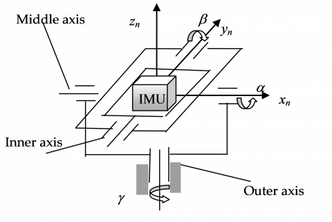
The initial mounting positions of the IMU in vertical and horizontal 3AT are displayed in Figures 1 and 2, respectively. Let γ, β and α be the angular positions of the outer, middle and inner axes of the 3AT, respectively.
Figure 1. The initial position of the IMU in vertical 3AT
As shown in Figure 1, the outer, middle and inner axes of the vertical 3AT rotate about axes zn, xn and yn, respectively. The attitude matrix of the IMU can be established as:
$\mathbf{C}_{b}^{n}=\text{Rot}(z,\gamma )\text{Rot}(x,\alpha )\text{Rot}(y,\beta )$ (7)
Thus, the input excitations of specific forces provided by the vertical 3AT to the accelerometers in the IMU can be described as:
${{\mathbf{f}}^{b}}=\mathbf{C}_{n}^{b}\left[ \begin{matrix} 0 \\ 0 \\ 1 \\\end{matrix} \right]=\left[ \begin{matrix} -\sin \beta \cos \alpha \\ \sin \alpha \\ \cos \beta \cos \alpha \\\end{matrix} \right]$ (8)
According to Eq. (8), when only the middle axis rotates on the vertical 3AT and belongs to the velocity state ($\alpha (t)=\omega t$), the accelerometers can receive alternating input of specific forces:
${{\mathbf{f}}^{b}}=\left[ \begin{matrix} -\sin \beta \cos \omega t \\ \sin \omega t \\ \cos \beta \cos \omega t \\\end{matrix} \right]$ (9)
Figure 2. The initial mounting position of the IMU in horizontal 3AT
As shown in Figure 2, the outer, middle and inner axes of the horizontal 3AT rotate about axes xn, zn and yn, respectively. The attitude matrix of the IMU can be established as:
$\mathbf{C}_{b}^{n}=\text{Rot}(x,\gamma )\text{Rot}(z,\alpha )\text{Rot}(y,\beta )$ (10)
Thus, the input excitations of specific forces provided by the horizontal 3AT to the accelerometers in the IMU can be described as:
${{\mathbf{f}}^{b}}=\left[ \begin{matrix} \sin \alpha \cos \beta \sin \gamma -\sin \beta \cos \gamma \\ cos\alpha \sin \gamma \\ sin\alpha sin\beta \sin \gamma +\cos \beta \cos \gamma \\\end{matrix} \right]$ (11)
According to equation (11), the accelerometers can receive alternating inputs of specific forces, when the middle axis or outer axis rotates in angular rate state. for example, $\gamma (t)=\omega t$ we have:
${{\mathbf{f}}^{b}}=\left[ \begin{matrix} \sin \alpha \cos \beta \sin \omega t-\sin \beta \cos \omega t \\ cos\alpha \sin \omega t \\ sin\alpha sin\beta \sin \omega t+\cos \beta \cos \omega t \\\end{matrix} \right]$ (12)
The following can be derived through the comparison between equations (9) and (12). Both turntables can output alternating excitations of specific forces, when the corresponding axis excite the velocity state. However, the excitations of specific force fb y in y direction of the vertical 3AT in equation (9) remains as sinωt, its amplitude is constant ‘1g’, while that of the horizontal 3AT in equation (12) is cosαsinω, its amplitude is gcosα, changing with the angular positions.
In this paper, the advantages of horizontal 3AT are fully utilized to stimulate the IMU errors. Systematic calibration was performed in calibrating these errors mounted on the horizontal 3AT, with the outer axis in the angular rate state and the middle and inner axes in the angular position state.
3.2 Equal interval rotation plan
Traditionally, the calibration design only aims to identify model coefficients and to draw up a simple and quick test plan. From the mathematical perspective, the modelling and identification of the IMU errors are essentially a regression analysis problem in statistics. Many rotation plans have been developed for the calibration of SINS, in the light of the data optimization methods for regression test plan design, including uniform rotation test plan and combined rotation test plan that are D-optimal or quasi-D-optimal.
When the angular rate of the outer axis is ω, its vector representation in b-frame is ω[1 0 0]T. Based on quasi-D-optimal criterion, the test points in the calibration plan were selected from the surface of the ω-radius, that is, the vertices of the inscribed regular polyhedron of the sphere.
If the inscribed regular tetrahedron is a regular one, the four vertices of the tetrahedron can be selected as the test points for IMU error calibration. First, the center of the regular tetrahedron needs to be placed at the center of the b-frame of the IMU on the horizontal 3AT. From the knowledge of the solid geometry, the coordinates of the four vertices are $(\frac{\sqrt{3}}{3},\frac{\sqrt{3}}{3},\frac{\sqrt{3}}{3})$, $(-\frac{\sqrt{3}}{3},-\frac{\sqrt{3}}{3},\frac{\sqrt{3}}{3})$, $(-\frac{\sqrt{3}}{3},\frac{\sqrt{3}}{3},-\frac{\sqrt{3}}{3})$ and $(\frac{\sqrt{3}}{3},-\frac{\sqrt{3}}{3},-\frac{\sqrt{3}}{3})$, respectively.
On each vertex, the outer axis should rotate four times at equal intervals of 90° (0°$\rightarrow$90°, 90°$\rightarrow$180°, 180°$\rightarrow$270° and 270°$\rightarrow$360°). In total, the outer axis needs to rotate 16 times throughout the calibration.
When the angular positions of the middle and inner axes are at α and β positions, respectively, the unit vector [1 0 0]T of the gyro’s angular velocity in the b-frame can be expressed as:
${{\left( \text{Rot}(z,\alpha )\text{Rot}(y,\beta ) \right)}^{\text{T}}}\left[ \begin{matrix} 1 \\ 0 \\ 0 \\\end{matrix} \right]=\left[ \begin{matrix} \cos \beta \cos \alpha \\ -\sin \alpha \\ \sin \beta \cos \alpha \\\end{matrix} \right]$ (13)
Taking the vertex $(\frac{\sqrt{3}}{3},-\frac{\sqrt{3}}{3},-\frac{\sqrt{3}}{3})$ for example, the following can be derived from Eq. (13):
$\left\{ \begin{align} & \cos \beta \cos \alpha =\frac{\sqrt{3}}{3} \\ & -\sin \alpha =-\frac{\sqrt{3}}{3} \\ & \sin \beta \cos \alpha =-\frac{\sqrt{3}}{3} \\ \end{align} \right.$ (14)
Thus, we have:
$\left\{\begin{array}{l}{\beta=315^{\circ}} \\ {\alpha=35.2644^{\circ}}\end{array} \text { or }\left\{\begin{array}{l}{\beta=135^{\circ}} \\ {\alpha=144.7356^{\circ}}\end{array}\right.\right.$ (15)
Similarly, two solutions can be obtained for each of the other three vertices of the regular tetrahedron. The solution that corresponds to the more uniform inputs of specific force before the rotation of the outer axis should be preserved. The angular positions of the middle and inner axes of the horizontal 3AT are listed in Table 1.
Table 1. The equal interval rotation plan
|
|
1 |
2 |
3 |
4 |
|
a |
215.2644° |
144.7356° |
215.2644° |
144.7356° |
|
b |
225° |
315° |
45° |
135° |
When the middle and inner axes of the horizontal 3AT are at the i-th angular positions αi, βi (i=1, 2, 3, 4), the attitude matrix of the initially aligned IMU in the body frame l relative to the navigation frame n after the first rotation of the outer axis (0°$\rightarrow$90°) can be expressed as:
$\mathbf{C}_{l}^{n}(i,1)=\text{Rot}(z,{{\alpha }_{i}})\text{Rot}(y,{{\beta }_{i}})$ (16)
Meanwhile, the attitude matrix of b-frame versus n-frame can be presented as:
$\boldsymbol{C}_{b}^{n}(i, 1)=\boldsymbol{A} \boldsymbol{C}_{l}^{n}(i, 1)$ (17)
where, $\mathbf{A}=\text{Rot}(x,\frac{\text{ }\!\!\pi\!\!\text{ }}{2})=\left[ \begin{matrix} 1 & 0 & 0 \\ 0 & 0 & -1 \\ 0 & 1 & 0 \\\end{matrix} \right]$.
Similarly, when the middle and inner axes are at the i-th angular positions, the attitude matrices after the second rotation of the outer axis (90°$\rightarrow$180°) can be expressed as:
$\mathbf{C}_{l}^{n}(i,2)=\mathbf{AC}_{l}^{n}(i,1)$, $\mathbf{C}_{b}^{n}(i,2)=\mathbf{AC}_{l}^{n}(i,2)$ (18)
When the middle and inner axes are at the i-th angular positions, the attitude matrices after the third rotation of the outer axis (180°$\rightarrow$270°) can be expressed as:
$\mathbf{C}_{l}^{n}(i,3)={{\mathbf{A}}^{2}}\mathbf{C}_{l}^{n}(i,1)$, $\mathbf{C}_{b}^{n}(i,3)=\mathbf{AC}_{l}^{n}(i,3)$ (19)
When the middle and inner axes are at the i-th angular positions, the attitude matrices after the fourth rotation of the outer axis (270°$\rightarrow$360°) can be expressed as:
$\mathbf{C}_{l}^{n}(i,4)={{\mathbf{A}}^{3}}\mathbf{C}_{l}^{n}(i,1)$, $\mathbf{C}_{b}^{n}(i,4)=\mathbf{AC}_{l}^{n}(i,4)$ (20)
From Eqns. (17)-(20), when the middle and inner axes are at the i-th angular positions, the attitude matrices after the j-th rotation of the outer axis can be expressed as:
$\left\{ \begin{align} & \mathbf{C}_{l}^{n}(i,j)=\left[ \begin{matrix} {{c}_{11}} & {{c}_{12}} & {{c}_{13}} \\ {{c}_{21}} & {{c}_{22}} & {{c}_{23}} \\ {{c}_{31}} & {{c}_{32}} & {{c}_{33}} \\\end{matrix} \right] \\ & \mathbf{C}_{b}^{n}(i,j)=\mathbf{AC}_{l}^{n}(i,j)=\left[ \begin{matrix} {{c}_{11}} & {{c}_{12}} & {{c}_{13}} \\ -{{c}_{31}} & -{{c}_{32}} & -{{c}_{33}} \\ {{c}_{21}} & {{c}_{22}} & {{c}_{23}} \\\end{matrix} \right] \\ \end{align} \right.$ (21)
In this way, the attitude matrices can be derived for each of the 16 rotations in the equal rotation test plan.
4.1 Analysis accelerometer’s errors
According to Eq. (5), the observable Y2 is partially affected by accelerometer’s errors, and partially by gyro’s errors. The two parts are respectively denoted as Y2a and Y2g:
$\begin{align} & {{\mathbf{Y}}_{2a}}=-\mathbf{C}_{b}^{n}\delta {{\mathbf{M}}_{a}}\mathbf{C}_{n}^{b}{{\mathbf{g}}^{n}}+\mathbf{C}_{b}^{n}{{\mathbf{B}}_{a}}+\text{ } \\ & \text{ }\left[ \begin{matrix} -{{\left[ -\mathbf{C}_{l}^{n}\delta {{\mathbf{M}}_{a}}\mathbf{C}_{n}^{l}{{\mathbf{g}}^{n}}+\mathbf{C}_{l}^{n}{{\mathbf{B}}_{a}} \right]}_{\text{H}}} \\ 0 \\\end{matrix} \right] \\ \end{align}$ (22)
Substituting the attitude matrices in Eq. (21) into the above equation, the expression of Y2a can be rewritten as:
$\begin{align} & {{\mathbf{Y}}_{2a}}=\left[ \begin{matrix} {{c}_{11}} & {{c}_{12}} & {{c}_{13}} \\ -{{c}_{31}} & -{{c}_{32}} & -{{c}_{33}} \\ {{c}_{21}} & {{c}_{22}} & {{c}_{23}} \\\end{matrix} \right]\left( \begin{matrix} \Delta {{K}_{ax}}{{c}_{21}}g+{{B}_{ax}} \\ {{M}_{ayx}}{{c}_{21}}g+\Delta {{K}_{ay}}{{c}_{22}}g+{{B}_{ay}} \\ {{M}_{azx}}{{c}_{21}}g+{{M}_{azy}}{{c}_{22}}g+\Delta {{K}_{az}}{{c}_{23}}g+{{B}_{az}} \\\end{matrix} \right)- \\ & \text{ }\left[ \begin{matrix} \left[ \begin{matrix} {{c}_{11}} & {{c}_{12}} & {{c}_{13}} \\ {{c}_{21}} & {{c}_{22}} & {{c}_{23}} \\\end{matrix} \right]\left[ \begin{matrix} \Delta {{K}_{ax}}{{c}_{31}}g+{{B}_{ax}} \\ {{M}_{ayx}}{{c}_{31}}g+\Delta {{K}_{ay}}{{c}_{32}}g+{{B}_{ay}} \\ {{M}_{azx}}{{c}_{31}}g+{{M}_{azy}}{{c}_{32}}g+\Delta {{K}_{az}}{{c}_{33}}g+{{B}_{az}} \\\end{matrix} \right] \\ 0 \\\end{matrix} \right] \\ \end{align}$ (23)
Based on the accelerometer’s errors and their vectors, Eq. (23) can be expanded as:
$\begin{align} & {{\mathbf{Y}}_{2a}}=\left[ \begin{matrix} {{c}_{11}}{{c}_{21}}-{{c}_{11}}{{c}_{31}} \\ -2{{c}_{21}}{{c}_{31}} \\ c_{21}^{2} \\\end{matrix} \right]g\Delta {{K}_{ax}}+\left[ \begin{matrix} {{c}_{12}}{{c}_{22}}-{{c}_{12}}{{c}_{32}} \\ -2{{c}_{22}}{{c}_{32}} \\ c_{22}^{2} \\\end{matrix} \right]g\Delta {{K}_{ay}}+\left[ \begin{matrix} {{c}_{13}}{{c}_{23}}-{{c}_{13}}{{c}_{33}} \\ -2{{c}_{23}}{{c}_{33}} \\ c_{23}^{2} \\\end{matrix} \right]g\Delta {{K}_{az}}+\left[ \begin{matrix} {{c}_{12}}{{c}_{21}}-{{c}_{12}}{{c}_{31}} \\ -{{c}_{21}}{{c}_{32}}-{{c}_{31}}{{c}_{22}} \\ {{c}_{21}}{{c}_{22}} \\\end{matrix} \right]g{{M}_{ayx}}+ \\ & \text{ }\left[ \begin{matrix} {{c}_{13}}{{c}_{21}}-{{c}_{13}}{{c}_{31}} \\ -{{c}_{21}}{{c}_{33}}-{{c}_{23}}{{c}_{31}} \\ {{c}_{21}}{{c}_{23}} \\\end{matrix} \right]g{{M}_{azx}}+\left[ \begin{matrix} {{c}_{13}}{{c}_{22}}-{{c}_{13}}{{c}_{32}} \\ -{{c}_{22}}{{c}_{33}}-{{c}_{23}}{{c}_{32}} \\ {{c}_{22}}{{c}_{23}} \\\end{matrix} \right]g{{M}_{azy}}+\left[ \begin{matrix} 0 \\ -{{c}_{32}}-{{c}_{22}} \\ {{c}_{22}} \\\end{matrix} \right]{{B}_{ay}}+\left[ \begin{matrix} 0 \\ -{{c}_{31}}-{{c}_{21}} \\ {{c}_{21}} \\\end{matrix} \right]{{B}_{ax}}\left[ \begin{matrix} 0 \\ -{{c}_{33}}-{{c}_{23}} \\ {{c}_{23}} \\\end{matrix} \right]{{B}_{az}} \\\end{align}$ (24)
The vector $\left[ \begin{matrix} {{c}_{11}}{{c}_{21}}-{{c}_{11}}{{c}_{31}} \\ -2{{c}_{21}}{{c}_{31}} \\ c_{21}^{2} \\\end{matrix} \right]g$ of the accelerometer error ∆Kax is denoted as ${{L}_{\Delta {{K}_{ax}}}}$ . The other error vectors are denoted in a similar manner.
The relationship between Y2a and the accelerometer’s errors to be calibrated can be observed clearly in Eq. (24).
4.2 Analysis on gyro’s errors
According to Eq. (5), the observable Y2g of the gyro’s errors can be described as:
$\begin{align} & {{\mathbf{Y}}_{2g}}=-\mathbf{C}_{l}^{n}\left\{ \frac{(1-\cos a)}{{{a}^{2}}}({{\mathbf{\sigma }}^{\times }}\cdot \delta {{\mathbf{\sigma }}^{\times }}+\delta {{\mathbf{\sigma }}^{\times }}\cdot {{\mathbf{\sigma }}^{\times }})+ \right. \\ & \text{ }\frac{\sin a}{a}\delta {{\mathbf{\sigma }}^{\times }}+\left( \frac{(a\cos a-\sin a){{\mathbf{\sigma }}^{\text{T}}}\delta \mathbf{\sigma }}{{{a}^{3}}}{{\mathbf{\sigma }}^{\times }} \right)+ \\ & \text{ }\left. \frac{(a\sin a-2(1-\cos a)){{\mathbf{\sigma }}^{\text{T}}}\delta \mathbf{\sigma }}{{{a}^{4}}}{{({{\mathbf{\sigma }}^{\times }})}^{2}} \right\}\mathbf{C}_{n}^{b}{{\mathbf{g}}^{n}} \\ \end{align}$ (25)
After the alignment of the IMU, the following can be derived through the equal interval rotation plan:
$\mathbf{\sigma }=\int_{0}^{{{T}_{1}}}{\mathbf{\omega }_{nb}^{b}}\text{d}t=\int_{0}^{{{T}_{1}}}{\mathbf{C}_{n}^{l}\cdot \left[ \begin{matrix} \omega \\ 0 \\ 0 \\\end{matrix} \right]}\text{d}t=\frac{\text{ }\!\!\pi\!\!\text{ }}{2}\left[ \begin{matrix} {{c}_{11}} \\ {{c}_{12}} \\ {{c}_{13}} \\\end{matrix} \right]\triangleq \frac{\text{ }\!\!\pi\!\!\text{ }}{2}\mathbf{m}$ (26)
$\delta \mathbf{\sigma }=\delta {{\mathbf{M}}_{g}}\mathbf{\sigma }+{{T}_{1}}{{\mathbf{B}}_{g}}=\frac{\text{ }\!\!\pi\!\!\text{ }}{2}\delta {{\mathbf{M}}_{g}}\mathbf{m}+{{T}_{1}}{{\mathbf{B}}_{g}}$ (27)
$a=\sqrt{\sigma _{x}^{2}+\sigma _{y}^{2}+\sigma _{z}^{2}}=\frac{\text{ }\!\!\pi\!\!\text{ }}{2}$ (28)
where, m=[c11, c12, c13]T. According to the nature of the direction cosine matrix, m is a unit vector satisfying mTm=1.
Substituting Eqns. (26)~(28) into Eq. (25), Y2g is expressed as:
$Y_{2 g}=-C_{l}^{n}\left\{\begin{array}{l}{\left(\delta M_{g} m+\frac{2}{\pi} T_{1} B_{g}\right)^{\times}} \\ {-m^{\mathrm{T}}\left(\delta M_{g} m+\frac{2}{\pi} T_{1} B_{g}\right) m^{\times}}\end{array}\right.\left(\begin{array}{c}{m^{\times}\left(\delta M_{g} m+\frac{2}{\pi} T_{1} B_{g}\right)^{\times}} \\ {+\left(\delta M_{g} m+\frac{2}{\pi} T_{1} B_{g}\right)^{x} m^{\times}}\end{array}\right)+\left.\left(\frac{\pi}{2}-2\right) \boldsymbol{m}^{\mathrm{T}}\left(\delta \boldsymbol{M}_{g} \boldsymbol{m}+\frac{2}{\pi} T_{1} \boldsymbol{B}_{g}\right)\left(\boldsymbol{m}^{\times}\right)^{2}\right\} \boldsymbol{C}_{n}^{b} \boldsymbol{g}^{n}$ (29)
The following properties of vectors are introduced to further analyze the Y2g of the gyro [19].
Lemma 1 For any two 3D vectors a and b, we have:
${{\mathbf{a}}^{\times }}{{\mathbf{b}}^{\times }}+{{\mathbf{b}}^{\times }}{{\mathbf{a}}^{\times }}=\mathbf{a}{{\mathbf{b}}^{\text{T}}}+\mathbf{b}{{\mathbf{a}}^{\text{T}}}-2{{\mathbf{a}}^{\text{T}}}\mathbf{b}\cdot \mathbf{I}$ (30)
Lemma 2 For any 3D vector a, we have:
${{({{\mathbf{a}}^{\times }})}^{2}}=\mathbf{a}{{\mathbf{a}}^{\text{T}}}-{{\mathbf{a}}^{2}}\mathbf{I}$ (31)
Based on Lemmas 1 and 2, Eq. (29) is expanded into:
$\begin{align} & {{\mathbf{Y}}_{2g}}=-\mathbf{C}_{l}^{n}\left\{ {{\left( \delta {{\mathbf{M}}_{g}}\mathbf{m} \right)}^{\times }}+\frac{2}{\text{ }\!\!\pi\!\!\text{ }}{{T}_{1}}\mathbf{B}_{g}^{\times }+\mathbf{m}{{\left( \delta {{\mathbf{M}}_{g}}\mathbf{m}+\frac{2}{\text{ }\!\!\pi\!\!\text{ }}{{T}_{1}}{{\mathbf{B}}_{g}} \right)}^{\text{T}}}+\left( \delta {{\mathbf{M}}_{g}}\mathbf{m}+\frac{2}{\text{ }\!\!\pi\!\!\text{ }}{{T}_{1}}{{\mathbf{B}}_{g}} \right){{\mathbf{m}}^{\text{T}}}- \right. \\ & 2{{\mathbf{m}}^{\text{T}}}\left( \delta {{\mathbf{M}}_{g}}\mathbf{m}+\frac{2}{\text{ }\!\!\pi\!\!\text{ }}{{T}_{1}}{{\mathbf{B}}_{g}} \right)\mathbf{I}-{{\mathbf{m}}^{\text{T}}}\left( \delta {{\mathbf{M}}_{g}}\mathbf{m}+\frac{2}{\text{ }\!\!\pi\!\!\text{ }}{{T}_{1}}{{\mathbf{B}}_{g}} \right){{\mathbf{m}}^{\times }}\left. +(\frac{\text{ }\!\!\pi\!\!\text{ }}{2}-2){{\mathbf{m}}^{\text{T}}}(\delta {{\mathbf{M}}_{g}}\mathbf{m}+\frac{2}{\text{ }\!\!\pi\!\!\text{ }}{{T}_{1}}{{\mathbf{B}}_{g}}){{({{\mathbf{m}}^{\times }})}^{2}} \right\}\mathbf{C}_{n}^{b}{{\mathbf{g}}^{n}}\text{ } \\ & \text{ }=-\mathbf{C}_{l}^{n}\left\{ {{\left( \delta {{\mathbf{M}}_{g}}\mathbf{m} \right)}^{\times }}+\frac{2}{\text{ }\!\!\pi\!\!\text{ }}{{T}_{1}}\mathbf{B}_{g}^{\times }+\mathbf{m}{{\mathbf{m}}^{\text{T}}}\delta \mathbf{M}_{g}^{\text{T}}+\frac{2}{\text{ }\!\!\pi\!\!\text{ }}{{T}_{1}}\mathbf{mB}_{g}^{\text{T}}+\delta {{\mathbf{M}}_{g}}\mathbf{m}{{\mathbf{m}}^{\text{T}}}+\frac{2}{\text{ }\!\!\pi\!\!\text{ }}{{T}_{1}}{{\mathbf{B}}_{g}}{{\mathbf{m}}^{\text{T}}}- \right. \\ & \text{ }\left. \text{ }{{\mathbf{m}}^{\text{T}}}\left( \delta {{\mathbf{M}}_{g}}\mathbf{m}+\frac{2}{\text{ }\!\!\pi\!\!\text{ }}{{T}_{1}}{{\mathbf{B}}_{g}} \right)\left( \frac{\text{ }\!\!\pi\!\!\text{ }}{2}\mathbf{I}+{{\mathbf{m}}^{\times }}+(2-\frac{\text{ }\!\!\pi\!\!\text{ }}{2})\mathbf{m}{{\mathbf{m}}^{\text{T}}} \right) \right\}\mathbf{C}_{n}^{b}{{\mathbf{g}}^{n}} \\ \end{align}$ (32)
It is learned from Eq. (32) that the Y2g is partially affected by mounting misalignment δMg and partially by biases Bg, both are gyro’s errors. Then, the observable can be expanded according to the corresponding errors.
Firstly, the relationship between Y2g and Bg can be derived from Eq. (32) as:
$\begin{align} & {{\mathbf{Y}}_{2g\_{{B}_{g}}}}=-\frac{2}{\text{ }\!\!\pi\!\!\text{ }}{{T}_{1}}\mathbf{C}_{l}^{n}\left[ \mathbf{B}_{g}^{\times }+\mathbf{mB}_{g}^{\text{T}}+{{\mathbf{B}}_{g}}{{\mathbf{m}}^{\text{T}}}- \right. \\ & \left. {{\mathbf{m}}^{\text{T}}}{{\mathbf{B}}_{g}}\left( \frac{\text{ }\!\!\pi\!\!\text{ }}{2}\mathbf{I}+{{\mathbf{m}}^{\times }}+(2-\frac{\text{ }\!\!\pi\!\!\text{ }}{2})\mathbf{m}{{\mathbf{m}}^{\text{T}}} \right) \right]\mathbf{C}_{n}^{b}{{\mathbf{g}}^{n}} \\ \end{align}$ (33)
Substituting Eq. (21) into Eq. (33), the vector of Bg in Y2g can be described as:
$\begin{align} & {{\mathbf{L}}_{{{B}_{gx}}}}=\frac{2}{\text{ }\!\!\pi\!\!\text{ }}{{T}_{1}}\left[ \begin{matrix} {{c}_{11}} & {{c}_{12}} & {{c}_{13}} \\ {{c}_{21}} & {{c}_{22}} & {{c}_{23}} \\ {{c}_{31}} & {{c}_{32}} & {{c}_{33}} \\\end{matrix} \right]\left\{ \left[ \begin{matrix} 2{{c}_{11}} & {{c}_{12}} & {{c}_{13}} \\ {{c}_{12}} & 0 & -1 \\ {{c}_{13}} & 1 & 0 \\\end{matrix} \right] \right.- \\ & \left. \text{ }{{c}_{11}}\left[ \begin{matrix} 2-(2-\frac{\text{ }\!\!\pi\!\!\text{ }}{2})(c_{12}^{2}+c_{13}^{2}) & -{{c}_{13}}+(2-\frac{\text{ }\!\!\pi\!\!\text{ }}{2}){{c}_{11}}{{c}_{12}} & {{c}_{12}}+(2-\frac{\text{ }\!\!\pi\!\!\text{ }}{2}){{c}_{11}}{{c}_{13}} \\ {{c}_{13}}+(2-\frac{\text{ }\!\!\pi\!\!\text{ }}{2}){{c}_{11}}{{c}_{12}} & 2-(2-\frac{\text{ }\!\!\pi\!\!\text{ }}{2})(c_{11}^{2}+c_{13}^{2}) & -{{c}_{11}}+(2-\frac{\text{ }\!\!\pi\!\!\text{ }}{2}){{c}_{12}}{{c}_{13}} \\ -{{c}_{12}}+(2-\frac{\text{ }\!\!\pi\!\!\text{ }}{2}){{c}_{11}}{{c}_{13}} & {{c}_{11}}+(2-\frac{\text{ }\!\!\pi\!\!\text{ }}{2}){{c}_{12}}{{c}_{13}} & 2-(2-\frac{\text{ }\!\!\pi\!\!\text{ }}{2})(c_{11}^{2}+c_{12}^{2}) \\\end{matrix} \right] \right\}\left[ \begin{matrix} {{c}_{21}} \\ {{c}_{22}} \\ {{c}_{23}} \\\end{matrix} \right]g \\ \end{align}$ (34)
The vectors of gyro biases Bgy and Bgz can be computed similarly.
According to Eq. (32), the relationship between Y2g and δMg can be depicted as:
\[\begin{align} & {{\mathbf{Y}}_{2g\_\delta Mg}}=-\mathbf{C}_{l}^{n}\left[ {{\left( \delta {{\mathbf{M}}_{g}}\mathbf{m} \right)}^{\times }}+\mathbf{m}{{\mathbf{m}}^{\text{T}}}\delta \mathbf{M}_{g}^{\text{T}}+\delta {{\mathbf{M}}_{g}}\mathbf{m}{{\mathbf{m}}^{\text{T}}}- \right. \\ & \left. {{\mathbf{m}}^{\text{T}}}\delta {{\mathbf{M}}_{g}}\mathbf{m}\left( \frac{\text{ }\!\!\pi\!\!\text{ }}{2}\mathbf{I}+{{\mathbf{m}}^{\times }}+(2-\frac{\text{ }\!\!\pi\!\!\text{ }}{2})\mathbf{m}{{\mathbf{m}}^{\text{T}}} \right) \right]\mathbf{C}_{b}^{n}{{\mathbf{g}}^{n}} \\ \end{align}\] (35)
Substituting Eq. (21) into Eq. (35), the vector of the scale factor ∆Kgxin Y2g_δMg can be described as:
$\begin{align} & {{\mathbf{L}}_{\Delta {{K}_{gx}}}}=\left[ \begin{matrix} {{c}_{11}} & {{c}_{12}} & {{c}_{13}} \\ {{c}_{21}} & {{c}_{22}} & {{c}_{23}} \\ {{c}_{31}} & {{c}_{32}} & {{c}_{33}} \\\end{matrix} \right]\left\{ \left[ \begin{matrix} 2c_{11}^{2} & {{c}_{11}}{{c}_{12}} & {{c}_{11}}{{c}_{13}} \\ {{c}_{11}}{{c}_{12}} & 0 & -{{c}_{11}} \\ {{c}_{11}}{{c}_{13}} & {{c}_{11}} & 0 \\\end{matrix} \right]- \right. \\ & \text{ }\left. c_{11}^{2}\left[ \begin{matrix} \frac{\text{ }\!\!\pi\!\!\text{ }}{2}+(2-\frac{\text{ }\!\!\pi\!\!\text{ }}{2})c_{11}^{2} & -{{c}_{13}}+(2-\frac{\text{ }\!\!\pi\!\!\text{ }}{2}){{c}_{11}}{{c}_{12}} & {{c}_{12}}+(2-\frac{\text{ }\!\!\pi\!\!\text{ }}{2}){{c}_{11}}{{c}_{13}} \\ {{c}_{13}}+(2-\frac{\text{ }\!\!\pi\!\!\text{ }}{2}){{c}_{11}}{{c}_{12}} & \frac{\text{ }\!\!\pi\!\!\text{ }}{2}+(2-\frac{\text{ }\!\!\pi\!\!\text{ }}{2})c_{12}^{2} & -{{c}_{11}}+(2-\frac{\text{ }\!\!\pi\!\!\text{ }}{2}){{c}_{12}}{{c}_{13}} \\ -{{c}_{12}}+(2-\frac{\text{ }\!\!\pi\!\!\text{ }}{2}){{c}_{11}}{{c}_{13}} & {{c}_{11}}+(2-\frac{\text{ }\!\!\pi\!\!\text{ }}{2}){{c}_{12}}{{c}_{13}} & \frac{\text{ }\!\!\pi\!\!\text{ }}{2}+(2-\frac{\text{ }\!\!\pi\!\!\text{ }}{2})c_{13}^{2} \\\end{matrix} \right] \right\}\left[ \begin{matrix} {{c}_{13}} \\ -{{c}_{33}} \\ {{c}_{23}} \\\end{matrix} \right]g \\ \end{align}$ (36)
The vectors of the other parameters in the gyro’s mounting misalignment matrix (Mgxy, Mgxz, Mgyx, ∆Mgy, Mgyz, Mgzx, Mgzy and ∆Mgz) can be computed in a similar manner.
Finally, the relationship between Y2g and gyro’s errors can be obtained with expanding the errors and their vectors with Eqns. (32) and (35):
$\begin{align} & {{\mathbf{Y}}_{2g}}=\frac{2}{\text{ }\!\!\pi\!\!\text{ }}{{T}_{1}}\left( \left[ \begin{matrix} {{d}_{1}} \\ {{d}_{2}} \\ {{d}_{3}} \\\end{matrix} \right]+{{c}_{11}}\left[ \begin{matrix} {{w}_{1}} \\ {{w}_{2}} \\ {{w}_{3}} \\\end{matrix} \right] \right)g\cdot {{B}_{gx}}+\frac{2}{\text{ }\!\!\pi\!\!\text{ }}{{T}_{1}}\left( \left[ \begin{matrix} {{s}_{1}} \\ {{s}_{2}} \\ {{s}_{3}} \\\end{matrix} \right]+{{c}_{12}}\left[ \begin{matrix} {{w}_{1}} \\ {{w}_{2}} \\ {{w}_{3}} \\\end{matrix} \right] \right)g\cdot {{B}_{gy}}+\frac{2}{\text{ }\!\!\pi\!\!\text{ }}{{T}_{1}}\left( \left[ \begin{matrix} {{m}_{1}} \\ {{m}_{2}} \\ {{m}_{3}} \\\end{matrix} \right]+{{c}_{13}}\left[ \begin{matrix} {{w}_{1}} \\ {{w}_{2}} \\ {{w}_{3}} \\\end{matrix} \right] \right)g\cdot {{B}_{gz}}\text{ }+ \\ & \text{ }\left( {{c}_{11}}\left[ \begin{matrix} {{d}_{1}} \\ {{d}_{2}} \\ {{d}_{3}} \\\end{matrix} \right]+c_{11}^{2}\left[ \begin{matrix} {{w}_{1}} \\ {{w}_{2}} \\ {{w}_{3}} \\\end{matrix} \right] \right)g\cdot \Delta {{K}_{gx}}+\left( {{c}_{12}}\left[ \begin{matrix} {{d}_{1}} \\ {{d}_{2}} \\ {{d}_{3}} \\\end{matrix} \right]+{{c}_{11}}{{c}_{12}}\left[ \begin{matrix} {{w}_{1}} \\ {{w}_{2}} \\ {{w}_{3}} \\\end{matrix} \right] \right)g\cdot {{M}_{gxy}}+\left( {{c}_{13}}\left[ \begin{matrix} {{d}_{1}} \\ {{d}_{2}} \\ {{d}_{3}} \\\end{matrix} \right]+{{c}_{11}}{{c}_{13}}\left[ \begin{matrix} {{w}_{1}} \\ {{w}_{2}} \\ {{w}_{3}} \\\end{matrix} \right] \right)g\cdot {{M}_{gxz}}\text{ }+ \\ & \text{ }\left( {{c}_{11}}\left[ \begin{matrix} {{s}_{1}} \\ {{s}_{2}} \\ {{s}_{3}} \\\end{matrix} \right]+{{c}_{11}}{{c}_{12}}\left[ \begin{matrix} {{w}_{1}} \\ {{w}_{2}} \\ {{w}_{3}} \\\end{matrix} \right] \right)g\cdot {{M}_{gyx}}+\left( {{c}_{12}}\left[ \begin{matrix} {{s}_{1}} \\ {{s}_{2}} \\ {{s}_{3}} \\\end{matrix} \right]+c_{12}^{2}\left[ \begin{matrix} {{w}_{1}} \\ {{w}_{2}} \\ {{w}_{3}} \\\end{matrix} \right] \right)g\cdot \Delta {{K}_{gy}}+\left( {{c}_{13}}\left[ \begin{matrix} {{s}_{1}} \\ {{s}_{2}} \\ {{s}_{3}} \\\end{matrix} \right]+{{c}_{12}}{{c}_{13}}\left[ \begin{matrix} {{w}_{1}} \\ {{w}_{2}} \\ {{w}_{3}} \\\end{matrix} \right] \right)g\cdot {{M}_{gyz}}\text{ }+ \\ & \text{ }\left( {{c}_{11}}\left[ \begin{matrix} {{m}_{1}} \\ {{m}_{2}} \\ {{m}_{3}} \\\end{matrix} \right]+{{c}_{11}}{{c}_{13}}\left[ \begin{matrix} {{w}_{1}} \\ {{w}_{2}} \\ {{w}_{3}} \\\end{matrix} \right] \right)g\cdot {{M}_{gzx}}+\left( {{c}_{12}}\left[ \begin{matrix} {{m}_{1}} \\ {{m}_{2}} \\ {{m}_{3}} \\\end{matrix} \right]+{{c}_{12}}{{c}_{13}}\left[ \begin{matrix} {{w}_{1}} \\ {{w}_{2}} \\ {{w}_{3}} \\\end{matrix} \right] \right)g\cdot {{M}_{gzy}}+\left( {{c}_{13}}\left[ \begin{matrix} {{m}_{1}} \\ {{m}_{2}} \\ {{m}_{3}} \\\end{matrix} \right]+c_{13}^{2}\left[ \begin{matrix} {{w}_{1}} \\ {{w}_{2}} \\ {{w}_{3}} \\\end{matrix} \right] \right)g\cdot \Delta {{K}_{gz}} \\ \end{align}$ (37)
where, ${{d}_{i}}={{c}_{i1}}(2{{c}_{11}}{{c}_{21}}+{{c}_{12}}{{c}_{22}}+{{c}_{13}}{{c}_{23}})+{{c}_{i2}}({{c}_{12}}{{c}_{21}}-{{c}_{23}})+{{c}_{i3}}({{c}_{13}}{{c}_{21}}+{{c}_{22}})$; ${{s}_{i}}={{c}_{i1}}({{c}_{11}}{{c}_{22}}+{{c}_{23}})+{{c}_{i2}}({{c}_{11}}{{c}_{21}}+2{{c}_{12}}{{c}_{22}}+{{c}_{13}}{{c}_{23}})+{{c}_{i3}}(-{{c}_{21}}+{{c}_{13}}{{c}_{22}})$; ${{m}_{i}}={{c}_{i1}}({{c}_{11}}{{c}_{22}}+{{c}_{23}})+{{c}_{i2}}({{c}_{11}}{{c}_{21}}+2{{c}_{21}}{{c}_{22}}+{{c}_{13}}{{c}_{23}})+{{c}_{i3}}(-{{c}_{21}}+{{c}_{13}}{{c}_{22}})$;
$\begin{align} & {{w}_{i}}={{c}_{i1}}\left[ \frac{\text{ }\!\!\pi\!\!\text{ }}{2}{{c}_{21}}+(2-\frac{\text{ }\!\!\pi\!\!\text{ }}{2})c_{11}^{2}{{c}_{21}}-{{c}_{13}}{{c}_{22}}+ \right.\text{ }\left. (2-\frac{\text{ }\!\!\pi\!\!\text{ }}{2}){{c}_{11}}{{c}_{12}}{{c}_{22}}+{{c}_{12}}{{c}_{23}}+(2-\frac{\text{ }\!\!\pi\!\!\text{ }}{2}){{c}_{11}}{{c}_{13}}{{c}_{23}} \right]+ \\ & \text{ }{{c}_{i2}}\left[ {{c}_{13}}{{c}_{21}}+(2-\frac{\text{ }\!\!\pi\!\!\text{ }}{2}){{c}_{11}}{{c}_{12}}{{c}_{21}}+\frac{\text{ }\!\!\pi\!\!\text{ }}{2}{{c}_{22}}+(2-\frac{\text{ }\!\!\pi\!\!\text{ }}{2})c_{12}^{2}{{c}_{22}}- \right.\left. {{c}_{11}}{{c}_{23}}+(2-\frac{\text{ }\!\!\pi\!\!\text{ }}{2}){{c}_{12}}{{c}_{13}}{{c}_{23}} \right]+ \\ & \text{ }{{c}_{i3}}\left[ -{{c}_{12}}{{c}_{21}}+(2-\frac{\text{ }\!\!\pi\!\!\text{ }}{2}){{c}_{11}}{{c}_{13}}{{c}_{21}}+{{c}_{11}}{{c}_{22}}+ \right.(2-\frac{\text{ }\!\!\pi\!\!\text{ }}{2}){{c}_{12}}{{c}_{13}}{{c}_{22}}\left. +\frac{\text{ }\!\!\pi\!\!\text{ }}{2}{{c}_{23}}+(2-\frac{\text{ }\!\!\pi\!\!\text{ }}{2})c_{13}^{2}{{c}_{23}} \right] \\ \end{align}$; i=1, 2, 3.
4.3 Errors calibration
According to Eqns. (24) and (37), Y2 can be written as an algebraic combination of IMU errors and their vectors:
$\begin{align} & {{\mathbf{Y}}_{2}}={{\mathbf{L}}_{\Delta {{K}_{ax}}}}\cdot \Delta {{K}_{ax}}+{{\mathbf{L}}_{{{B}_{ax}}}}\cdot {{B}_{ax}}+{{\mathbf{L}}_{{{M}_{ayx}}}}\cdot {{M}_{ayx}}+{{\mathbf{L}}_{\Delta {{K}_{ay}}}}\cdot \Delta {{K}_{ay}} \\ & +{{\mathbf{L}}_{{{B}_{ay}}}}\cdot {{B}_{ay}}+{{\mathbf{L}}_{{{M}_{azx}}}}\cdot {{M}_{azx}}+{{\mathbf{L}}_{{{M}_{azy}}}}\cdot {{M}_{azy}}+{{\mathbf{L}}_{\Delta {{K}_{ay}}}}\cdot \Delta {{K}_{az}}+ \\ & \text{ }{{\mathbf{L}}_{{{B}_{az}}}}\cdot {{B}_{az}}+{{\mathbf{L}}_{{{B}_{gx}}}}\cdot {{B}_{gx}}+{{\mathbf{L}}_{{{B}_{gy}}}}\cdot {{B}_{gy}}+{{\mathbf{L}}_{{{B}_{gz}}}}\cdot {{B}_{gz}} \\ & +{{\mathbf{L}}_{\Delta {{K}_{gx}}}}\cdot \Delta {{K}_{gx}}+{{\mathbf{L}}_{{{M}_{gxy}}}}\cdot {{M}_{gxy}}+{{\mathbf{L}}_{{{M}_{gxz}}}}\cdot {{M}_{gxz}}+ \\ & \text{ }{{\mathbf{L}}_{\Delta {{K}_{gy}}}}\cdot \Delta {{K}_{gy}}+{{\mathbf{L}}_{{{M}_{gyx}}}}\cdot {{M}_{gyx}}+{{\mathbf{L}}_{{{M}_{gyz}}}}\cdot {{M}_{gyz}} \\ & +{{\mathbf{L}}_{{{M}_{gzx}}}}\cdot {{M}_{gzx}}+{{\mathbf{L}}_{{{M}_{gzy}}}}\cdot {{M}_{gzy}}+{{\mathbf{L}}_{\Delta {{K}_{gz}}}}\cdot \Delta {{K}_{gz}} \\ \end{align}$ (38)
Let Ls be the vector of an error, with s being the serial number of IMU error. By definition, Ls is an algebraic combination of the elements cij(i, j=1, 2, 3) in the attitude matrix. When it rotates to different attitudes, the horizontal 3AT provides the IMU with different input excitations, leading to different vectors of each IMU error.
After implementing the equal interval rotation plan, the observable Y2(i) (i=1,2,¼,16) under the simulation of the 16 rotations can be obtained by fitting the IMU velocities. When the outer axis rotates for the j-th time with the middle and inner axes at the i-th angular positions, the vector of each IMU error can be derived from the corresponding attitude matrices in Eqns. (17)~(20), and denoted as Ls(i,j).
Therefore, equation (38) can be expressed as the matrix below:
${{\mathbf{{Y}'}}_{2}}=\mathbf{\Phi K}$ (39)
where, ${{\mathbf{{Y}'}}_{2}}=\left[ \begin{matrix} \mathbf{Y}_{2}^{\text{T}}(1) & \cdots & \mathbf{Y}_{2}^{\text{T}}(n) \\\end{matrix} \right]_{3n\times 1}^{\text{T}}$; $\mathbf{K}=\left[ \begin{matrix} {{\mathbf{K}}_{A}} & {{\mathbf{K}}_{G}} \\\end{matrix} \right]_{21\times 1}^{\text{T}}$; $\mathbf{\Phi }={{\left[ \begin{matrix} {{\mathbf{\Phi }}_{A}}(1,1) & {{\mathbf{\Phi }}_{G}}(1,1) \\ \vdots & \vdots \\ {{\mathbf{\Phi }}_{A}}(4,4) & {{\mathbf{\Phi }}_{G}}(4,4) \\\end{matrix} \right]}_{3n\times 21}}$,
${{\mathbf{K}}_{A}}={{\left[ \begin{matrix} \Delta {{K}_{ax}} & {{B}_{ax}} & {{M}_{ayx}} & \Delta {{K}_{ay}} & {{B}_{ay}} & {{M}_{azx}} & {{M}_{azy}} & \Delta {{K}_{az}} & {{B}_{az}} \\\end{matrix} \right]}_{1\times 9}}$
${{\mathbf{K}}_{G}}={{\left[ \begin{matrix} {{B}_{gx}} & {{B}_{gy}} & {{B}_{gz}} & \Delta {{K}_{gx}} & {{M}_{gxy}} & {{M}_{gxz}} & \Delta {{K}_{gy}} & {{M}_{gyx}} & {{M}_{gyz}} & {{M}_{gzx}} & {{M}_{gzy}} & \Delta {{K}_{gz}} \\\end{matrix} \right]}_{1\times 12}}$
${{\mathbf{\Phi }}_{A}}(i,j)={{\left[ \begin{matrix} {{\mathbf{L}}_{\Delta {{K}_{ax}}}}(i,j) & {{\mathbf{L}}_{{{B}_{ax}}}}(i,j) & {{\mathbf{L}}_{{{M}_{ayx}}}}(i,j) & {{\mathbf{L}}_{\Delta {{K}_{ay}}}}(i,j) & {{\mathbf{L}}_{{{B}_{ay}}}}(i,j) & {{\mathbf{L}}_{{{M}_{azx}}}}(i,j) & {{\mathbf{L}}_{{{M}_{azy}}}}(i,j) & {{\mathbf{L}}_{\Delta {{K}_{az}}}}(i,j) & {{\mathbf{L}}_{{{B}_{az}}}}(i,j) \\\end{matrix} \right]}_{3\times 9}}$
$\begin{align} & {{\mathbf{\Phi }}_{G}}(i,j)=\left[ \begin{matrix} {{\mathbf{L}}_{{{B}_{gx}}}}(i,j) & {{\mathbf{L}}_{{{B}_{gy}}}}(i,j) & {{\mathbf{L}}_{{{B}_{gz}}}}(i,j) & {{\mathbf{L}}_{\Delta {{K}_{gx}}}}(i,j) & {{\mathbf{L}}_{{{M}_{gxy}}}}(i,j) & {{\mathbf{L}}_{{{M}_{gxz}}}}(i,j) & {{\mathbf{L}}_{{{M}_{gyx}}}}(i,j) & {{\mathbf{L}}_{\Delta {{K}_{gy}}}}(i,j) & {{\mathbf{L}}_{{{M}_{gyz}}}}(i,j) \\\end{matrix} \right. \\ & \text{ }{{\left. \begin{matrix} {{\mathbf{L}}_{{{M}_{gzx}}}}(i,j) & {{\mathbf{L}}_{{{M}_{gzy}}}}(i,j) & {{\mathbf{L}}_{\Delta {{K}_{gz}}}}(i,j) \\\end{matrix} \right]}_{3\times 12}} \\ & \text{ } \\ \end{align}$ n=16; i, j=1, 2, 3, 4.
The vectors K can be obtained by processing Eq. (39) with the least square method:
$\mathbf{K}={{({{\mathbf{\Phi }}^{\text{T}}}\mathbf{\Phi })}^{-1}}{{\mathbf{\Phi }}^{\text{T}}}{{\mathbf{{Y}'}}_{2}}$ (40)
The above equation shows that the systematic calibration model can identify all IMU errors, after implementing the equal interval rotation plan.
Let ΦTΦ=A be the information matrix. Then, the uncertainties of each IMU error can be expressed as:
$\left\{ \begin{align} & \sigma (\Delta {{K}_{ax}})=\sigma ({{\mathbf{Y}}_{2}}^{\prime })\sqrt{{{a}_{1,1}}^{2}+{{a}_{1,2}}^{2}+\cdots +{{a}_{1,3n}}^{2}} \\ & \sigma ({{B}_{ax}})=\sigma ({{\mathbf{Y}}_{2}}^{\prime })\sqrt{{{a}_{2,1}}^{2}+{{a}_{2,2}}^{2}+\cdots +{{a}_{2,3n}}^{2}} \\ & \text{ }\cdots \cdots \cdots \cdots \cdots \\ & \sigma ({{M}_{gzy}})=\sigma ({{\mathbf{Y}}_{2}}^{\prime })\sqrt{{{a}_{20,1}}^{2}+{{a}_{20,2}}^{2}+\cdots +{{a}_{20,3n}}^{2}} \\ & \sigma (\Delta {{K}_{gz}})=\sigma ({{\mathbf{Y}}_{2}}^{\prime })\sqrt{{{a}_{21,1}}^{2}+{{a}_{21,2}}^{2}+\cdots +{{a}_{21,3n}}^{2}} \\ \end{align} \right.$ (41)
The information matrix A for the calibration path can be derived from the attitude matrices at the 16 rotation positions of the equal interval rotation plan, revealing the uncertainty of each IMU error according to that plan.
If the random errors of the accelerometers in IMU all are 10μg (1σ), and the random errors of the gyros are all 0.01°/h (1σ), the standard deviations resulting in Y2’ as 10-4m/s2 according to Eq. (5). From Eq. (41), the scale factors and the uncertainties of the biases for the accelerometers in the IMU can be obtained as:
$\left\{\begin{array}{l}{\sigma\left(\Delta K_{a x}\right)=1.6868 \mathrm{pm}} \\ {\sigma\left(\Delta K_{a x}\right)=1.9752 \mathrm{pm}} \\ {\sigma\left(\Delta K_{a x}\right)=1.5603 \mathrm{pm}} \\ {\sigma\left(B_{a x}\right)=9.9297 \mathrm{ug}} \\ {\sigma\left(B_{a y}\right)=9.9297 \mathrm{lug}} \\ {\sigma\left(B_{x}\right)=9.9298 \mathrm{Hg}}\end{array}\right.$; $\left\{\begin{array}{l}{\sigma\left(\Delta K_{g x}\right)=1.7244 \mathrm{pm}} \\ {\sigma\left(\Delta K_{g y}\right)=1.7581 \mathrm{ppm}} \\ {\sigma\left(\Delta K_{g z}\right)=1.3460 \mathrm{ppm}} \\ {\sigma\left(B_{g x}\right)=0.0037 \%} \\ {\sigma\left(B_{g y}\right)=0.0035^{\circ} / \mathrm{h}} \\ {\sigma\left(B_{g z}\right)=0.0036^{\circ} / \mathrm{h}}\end{array}\right.$ (42)
Eqns. (41) and (42) show that the calibration accuracy of IMU errors is affected directly by the standard deviations of the 16 observed quantities Y2’ and the information matrix A, and indirectly by the design of the equal interval rotation plan through the information matrix A. The calibration accuracy of the IMU errors through the equal interval rotation plan is verified through the following simulation.
Our systematic calibration method and separated calibration method were both applied to identify the IMU errors. The calibration scheme is shown in Table 1. The preset errors and calibration errors (calibration error= preset error – calibration result) are listed in Table 2.
The simulation conditions include gravitational acceleration g=9.8m/s2; turn rate of the Earth wie=15.04107 °/h; local latitude L=45°; angular position error of horizontal 3AT 1²; angular velocity of outer axis 1°/s; the random errors of the accelerometers in IMU all are10μg; the random errors of the gyros all are 0.01°/h.
This systematic calibration method was simulated on Matlab in the following steps:
Step 1. Alignment: The SINS was subjected to initial alignment.
Step 2. Rotations: The SINS entered the navigation mode. The angular positions of the middle and inner axes of the horizontal 3AT were adjusted as per the calibration scheme, such that the IMU reached the four vertices of the regular tetrahedron in turns. Then, the outer axis rotated four times at equal intervals of 90° on each vertex (0°®90°, 90°®180°, 180°®270° and 270°®360°).
Step 3. Stationary measurement: After each rotation, the errors were measured in stationary state and then the navigation mode was terminated.
Step 4. Data collection: The IMU’s attitude, velocity and position were computed under the simulation of the 16 rotations in the equal interval rotation plan. The velocity error δVn en was fitted by quadratic function, and the coefficient of the second-order term Y1 was taken as the observable.
Step 5. Error calibration: The IMU errors were calibrated by equation (4), and the calibration error for IMU’s each error was computed.
The traditional separated calibration method only requires the initial alignment of the IMU. Then, the accelerometer errors were calibrated based on the static positions before the 16 rotations in the test plan, and the gyro’s errors were calibrated based on the angular velocities of the 16 rotations.
Table 2. Comparison of simulation results of the two calibration methods
|
IMU parameters |
Simulation preset value |
Calibration error of Systematic |
Calibration error of Separation |
IMU parameters |
Simulation preset value |
Calibration error of Systematic |
Calibration error of Separation |
|
DKax (ppm) |
200 |
-0.065 |
4.1787 |
DKgx(ppm) |
600 |
0.6997 |
-2.7083 |
|
DKay (ppm) |
400 |
-0.0547 |
2.5267 |
DKgy(ppm) |
-300 |
0.5981 |
6.9736 |
|
DKaz(ppm) |
-300 |
0.065 |
-5.8407 |
DKgz(ppm) |
100 |
-0.5748 |
-3.2387 |
|
Bax(μg) |
600 |
-6.5207 |
-1.9437 |
Bgx(°/h) |
-0.7 |
-0.0039 |
-0.0094 |
|
Bay(μg) |
200 |
-7.3282 |
-1.9412 |
Bgy(°/h) |
0.2 |
0.0019 |
0.023 |
|
Baz(μg) |
-300 |
-1.8958 |
-0.6687 |
Bgz(°/h) |
0.5 |
0.0022 |
-0.0061 |
|
Mayx (¢) |
2 |
0.0026 |
0.0143 |
Mgxy(¢) |
5 |
-0.0008 |
0.0171 |
|
Mazx(¢) |
2 |
0 |
0.0039 |
Mgxz(¢) |
5 |
-0.0003 |
-0.0203 |
|
Mazy(¢) |
2 |
0.0085 |
0.0038 |
Mgyx(¢) |
5 |
0.0041 |
-0.0072 |
|
—— |
—— |
—— |
—— |
Mgyz(¢) |
5 |
-0.0121 |
0.0032 |
|
—— |
—— |
—— |
—— |
Mgzx(¢) |
5 |
0.0003 |
-0.0173 |
|
—— |
—— |
—— |
—— |
Mgzy(¢) |
5 |
-0.0053 |
0.0164 |
Table 2 lists the calibration errors of the two calibration methods for the IMU errors. The systematic calibration obviously outperformed the separated calibration. The systematic calibration was almost one order of magnitude higher than the separated calibration in terms of the scale factors and mounting misalignments of the accelerometers and gyros, as well as the gyros biases. For systematic calibration, the calibration error of the gyros biases was 0.0039°/h, better than the measurement noise (0.01°/h); the calibration error of the gyro’s mounting misalignment was controlled within 1², comparable to that of precision 3AT; the calibration error of the accelerometers biases was within 7.3mg, better than the measurement noise of the accelerometer, although not much better than that of separated calibration. To sum up, the separated calibration was less accurate than systematic calibration, because the observable Y2 in velocity error of this method was easily affected by the turntable error and ground velocity component.
The 100 Monte-Carlo (M-C) simulation tests were conducted fully to determine the calibration errors of the systematic calibration method concerning IMU errors. Based on the calibration errors of the 100 tests, the mean square errors (MSEs) of the scale factors and biases of the IMU were obtained (Table 3).
The systematic calibration results in Table 3 show that the calibration errors of the scale factors of the accelerometer and gyro were smaller than 0.53ppm and 4.4ppm, respectively, the calibration errors of the accelerometers biases smaller than 3.65mg, and that of the gyro was below 0.004°/h. These data were mostly on the same order of magnitude with the uncertainties of these errors obtained by Eq. (41). The simulation result on the accelerometers scale factor differed from the theoretical result by one order of magnitude, but the two results overlapped each other by 0.3 %, indicating that the calibration is accurate. The simulation results in Table 3 further validate the theoretical analysis on the identification accuracy of IMU errors.
Table 3. Calibration errors of the 100 M-C simulation tests based with systematic calibration method
|
IMU parameters |
uncertainty |
IMU parameters |
uncertainty |
|
DKax(ppm) |
0.2127 |
DKgx(ppm) |
2.6143 |
|
DKay(ppm) |
0.5294 |
DKgy(ppm) |
2.6200 |
|
DKaz(ppm) |
0.2127 |
DKgz(ppm) |
4.3669 |
|
Bax(μg) |
3.5042 |
Bgx (°/h) |
0.0039 |
|
Bay(μg) |
2.9160 |
Bgy(°/h) |
0.0033 |
|
Baz(μg) |
3.6443 |
Bgy(°/h) |
0.0032 |
To clearly describe the calibration results, the IMU was subjected to a 24h pure inertial navigation simulation under static position based on the results of the systematic calibration method and the separated calibration method. The static position was set to the initial position of the turntable, that is, the middle, inner and outer axes are all in 0 positions. The navigation errors are displayed in Figures 3-6.
Figure 3. Velocity errors of systematic calibration
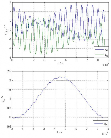
Figure 4. Attitude errors of systematic calibration
Figure 5. Velocity errors of separated calibration
Figure 6. Attitude errors of separated calibration
Comparing Figures 4 and 6, the attitude errors of systematic calibration peaked at 6² in the x- and y-directions, and 2.2¢ in the z-direction, while the attitude errors of separated calibration peaked at 23² in the x- and y-directions, and 8.2¢ in the z-direction. Comparing Figures 3 and 5, the maximum velocity error of systematic calibration was smaller than 0.3m/s, while that of separated calibration was larger than 1.5m/s. The above analysis demonstrates that the systematic calibration is more accurate than separated calibration, and that our method can effectively enhance navigation accuracy.
To effectively calibrate the IMU errors, this paper designed an equal interval rotation plan according to the relationship between IMU’s errors and velocity errors output by navigation algorithm of IMU,. and identified all IMU errors by the least square method. The simulation results show that, when the accuracies of accelerometer and gyro in the IMU are 10μg and 0.01°/h, respectively, the calibration uncertainty of the accelerometers biases was 3.65mg and the gyro’s biases was 0.004°/h. Besides, this method was compared with separated calibration method through a 24h pure inertial navigation simulation under static position. The comparison shows that this method reduced the calibration error of velocity by 1/5 and that of attitude by nearly 1/4 from the level of separated calibration, indicating that this method can effectively enhance the calibration accuracies of IMU errors.
The 13th Five-year Pre-research Foundation (4141708031); National Natural Science Foundation of China (61703123).
[1] Pan, J., Zhang, C., Niu, Y., Fan, Z. (2014). Accurate calibration for drift of fiber optic gyroscope in multi-position north-seeking phase. Optik-International Journal for Light and Electron Optics, 125(24): 7244-7246. https://doi.org/10.1016/j.ijleo.2014.07.126
[2] Lv, P., Lai J., Liu J., Nie, M. (2014). The compensation effects of gyros' stochastic errors in a rotational inertial navigation system. Journal of Navigation, 67(6): 1069-1088. https://doi.org/10.1017/S0373463314000319
[3] Fontanella, R., Accardo, D., Lo Moriello, R.S., Angrisani L., De Simonec, D. (2018). MEMS gyros temperature calibration through artificial neural networks. Sensors and Actuators A-Physical, 279(8): 553-565. https://doi.org/10.1016/j.sna.2018.04.008
[4] Ahmed, H., Tahir, M. (2017). Accurate attitude estimation of a moving land vehicle using low-cost mems IMU sensors. IEEE Transactions on Intelligent Transportation Systems, 18(7): 1723-1739. https://doi.org/10.1109/TITS.2016.2627536
[5] Fokin, L.A., Shchipitsin, A.G. (2008). Strapdown inertial navigation systems for high precision near-Earth navigation and satellite geodesy: Analysis of operation and errors. Journal of Computer and Systems Sciences International, 47(3): 485-497. https://doi.org/10.1134/s1064230708030180
[6] Nemec, D., Janota, A., Hruboš, M., Šimák, V. (2016). Intelligent real-time MEMS sensor fusion and calibration. IEEE Sensors Journal, 16(19): 7150-7160. https://doi.org/10.1109/JSEN.2016.2597292
[7] Nourmohammadi, H., Keighobadi, J. (2017). Decentralized INS/GPS system with MEMS-grade inertial sensors using QR-factorized CKF. IEEE Sensors Journal, 17(11): 3278-3287. https://doi.org/10.1109/JSEN.2017.2693246
[8] Wang, X. (2009). Fast alignment and calibration algorithms for inertial navigation system. Aerospace Science & Technology, 13(4-5): 204-209. https://doi.org/10.1016/j.ast.2009.04.002
[9] Hwangbo, M., Kim, J.S., Kanade, T. (2013). IMU self-calibration using factorization. IEEE Transactions on Robotics, 29(2): 493-507. https://doi.org/10.1109/TRO.2012.2230994
[10] Gao, W., Zhang, Y., Wang, J. (2015). Research on initial alignment and self-calibration of rotary strapdown inertial navigation systems. Sensors, 15(2): 3154-3171. https://doi.org/10.3390/s150203154
[11] Jurman, D., Jankovec, M., Kamnik, R., Topič, M. (2007). Calibration and data fusion solution for the miniature attitude and heading reference system. Sensors & Actuators a Physical, 138(2): 411-420. https://doi.org/10.1016/j.sna.2007.05.008
[12] Wang, L., Wang, W., Zhang, Q., Gao, P. (2014). Self-calibration method based on navigation in high-precision inertial navigation system with fiber optic gyro. Optical Engineering, 53(6): 64-103. https://doi.org/10.1117/1.OE.53.6.064103
[13] Wang, B., Ren, Q., Deng, Z.H., Fu, M. (2015). A self-calibration method for non-orthogonal angles between gimbals of rotational inertial navigation system. IEEE Trans. Industr. Electron, 62(4), 2353-2362. https://doi.org/10.1109/TIE.2014.2361671
[14] Rogers, R.M. (2015). In Applied Mathematics in Integrated Navigation Systems. Reston American Institute of Aeronautics & Astronautics Inc, USA, 78-82. https://doi.org/10.2514/4.861598
[15] Strachan, V.F. (2000). Inertial measurement technology in the satellite navigation environment. Journal of Navigation, 53(2): 247-260. https://doi.org/10.1017/S0373463300008808
[16] Nemec, D., Janota, A., Hruboš, M., Šimák, V. (2016). Intelligent real-time mems sensor fusion and calibration. IEEE Sensors Journal, 16(19): 7150-7160. https://doi.org/10.1109/JSEN.2016.2597292
[17] Lee, T.G., Sung, C.K. (2004). Estimation technique of fixed sensor errors for SDINS calibration. International Journal of Control, Automation and Systems, 2(4): 536-541.
[18] Rogers, R.M. (2007). Applied Mathematics in Integrated Navigation Systems. American Institute of Aeronautics and Astronautics, Inc, 46-70. https://doi.org/10.1080/0020739700010302
[19] Savage, P.G. (2008). Strapdown Analytics. Maple Plain, Minnesota: Strapdown Associates, Inc, 56-69.
[20] Yang, X., Huang, Y. (2008). Systematic calibration method for laser gyro SINS. Journal of Chinese Inertial Technology, 16(1): 1-7.
[21] Wu, H., Xiao, Z., Zhou, D., Wang, L. (2018). SINS installation error matrix decoupling method based on matrix decomposition. Systems Engineering and Electronics, 40(5): 1091-1097.