Abdelkrim Rechach* | Sihem Ghoudelbourk | Mihoub Mohamed Larbi
© 2022 IIETA. This article is published by IIETA and is licensed under the CC BY 4.0 license (http://creativecommons.org/licenses/by/4.0/).
OPEN ACCESS
The exploitation of solar energy and the universal interest in photovoltaic systems have increased nowadays due to galloping energy consumption and current geopolitical and economic issues. This has led to high technical and economic requirements. The PV system still faces major obstacles such as high cost and low efficiency compared to other renewable technologies. In addition, the photovoltaic system suffers from the rate of undesirable harmonics of the generated power which could alter the quality of energy and the performance requested by users. In order to remedy this problem, the use of the multi-level inverter is in these cases one of the most promising solutions. Indeed, the multi-level technology seems to be well suited to photovoltaic applications to help fill the need for several sources on the DC side of the converter. The technical performance and reliability of the multi-level inverter used to connect the PV modules to the electrical power distribution networks can improve and make profitable the power produced. In this work, we compare two multi-level inverter topologies for PV systems: H-Bridge (HB) and Neutral Point Clamped (NPC). The comparison between these inverters is based on the criteria of spectral quality of the output voltage and the complexity of the power circuits.
multilevel inverter, neutral point clamped (NPC), cascaded H-Bridge (HB), photovoltaic generator, total harmonic distortion (THD)
In view of the expected depletion of natural energy resources, environmental problems caused by the emission of greenhouse gases and current geopolitical issues, the use of renewable energy resources has become a necessity due to the fact that it presents an interesting alternative offering the possibility of producing clean electricity on the condition of adapting to their random natural fluctuations.
Photovoltaic energy is the most attractive among the various renewable energy sources due to the availability of free solar energy everywhere, the reliability of PV systems and the modularity of power according to need. The growth rate in this field is mainly due to installations connected to electrical distribution networks and to unprecedented progress in power electronics. However, the high cost, the low efficiency compared to other technologies and the unwanted harmonics in the power produced are handicaps for the PV system. This is a serious concern to be able to integrate PV systems into the grid. Improving power quality using a multi-level inverter is an attractive solution for multi-sources on the DC side of the converter for photovoltaic applications [1, 2].
Increasing the level of the inverter results a good voltage waveform and lower THD. However, the choice of the technical performance and the reliability of the multi-level inverter used for the connection of the PV modules to the electrical distribution networks can influence the quantity of electrical energy produced and the financial profitability of such a system. Connecting multiple PVs to the power grid through multi-level inverters reduces the total harmonic distortion (THD), thereby improving power quality. Their use proves to be an optimal solution for the connection of the PV system to the electrical networks and make it possible to increase the power delivered by the photovoltaic generator. The use of the latter makes it possible to simultaneously solve the difficulties linked to the clutter and to the control of groups of two-level inverters generally used in this type of application [3]. In this article, we present a comparison between two multi-level inverter topologies: H-Bridge (HB) and Neutral Point Clamped (NPC) for grid-connected PV systems.
Each inverter is controlled by the same type of control "sinusoidal pulse width modulation (SPWM)". The voltage sources supplying the inverters are direct voltage photovoltaic (PV) panels. We chose the 5L inverter because it is the most common.
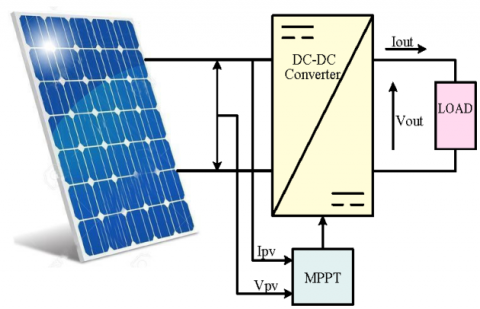
The selected electrical characteristics of the photovoltaic module (MSX60) are illustrated in Table 1 shown below. Figure 1 shows the block diagram of the PV system, made up of photovoltaic panels that transform solar energy into direct current which will be collected and then sent to the DC/DC converter. The latter, equipped with an MPPT algorithm, optimizes the power collected by stabilizing it at its maximum before delivering it to the load. The PV generator is made of mono-crystalline silicon and consists of 36 elementary photovoltaic cells. Under standard test conditions (CST= illumination G=1,000W/m², and Standard temperature T=25℃), it can deliver, a power of 60 W, a current of 3.5 A under an optimum voltage of 17.1 V. The adaptation quadrupole is an energy converter of the step-up for applications requiring voltages above 17 V.
Table 1. Electrical characteristics of the photovoltaic module MSX60
|
Characteristics |
Values |
|
Standard illumination, G |
1000 W/m² |
|
Standard temperature, T |
25℃ |
|
Maximum power, Pmax |
60 w |
|
Voltage at Pmax or optimum Voltage (Vopt) |
17.1 V |
|
Current to Pmax or optimal Current (Iopt) |
3.5 A |
|
Short-circuit current (Isc) |
3.8 A |
|
Open circuit voltage (Vco) |
21.1 V |
|
Number of cells in series |
36 |
|
Energy of the forbidden band |
1.12 ev |
|
Temperature coefficient of (Isc) |
65 mA /℃ |
|
Temperature coefficient of (Vco) |
-80 mA /℃ |
|
Temperature coefficient of power |
(0.5±0.05) %℃ |
|
Current power of saturation (Isat) |
20 nA |
Figure 1. Synoptic diagram of a system Photovoltaic controlled by MPPT
The Maximum Power Point Tracking (MPPT) control is a functional component of the PV system that helps to find the optimum operating point of the PV generator. For this, we chose to use the Perturbation and Observation (P&O) algorithm for its simplicity, which shifts the operating point to the point of maximum power periodically increasing or decreasing the voltage of the PV generator.
As shown in the Figure 2, if we cause a slight disturbance of the voltage, this produces a variation of the power. A positive change in the voltage ΔV>0 generates an increase in the power ΔP>0; this means that the operating point is to the left of the MPP. The reasoning is similar if the voltage decreases. It is therefore easy to locate the MPP. The purpose of the MPPT is to converge the voltage to the maximum power through an appropriate control command. The use of a microprocessor is more appropriate for the realization of the P&O algorithm, even if analog circuits can do it. The Figure 7 represents the classic algorithm of a P&O type MPPT control, where the evolution of the power is analyzed after each voltage disturbance.
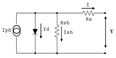
Figure 3 shows the electric model of a solar cell which consists of an ideal current source, connected with a series resistor Rs and a shunt resistor Rsh in parallel [3, 4]. The diode D describes the semiconductor properties of the cell. This model with an empirical diode) is currently the most used because of its simplicity.
Figure 2. Working principle of MPPT control
Figure 3. Equivalent circuit of a PV cell
Rsh showsleakage around the p-n junction due to impurities and cell corners, and Rs shows the internal resistance of the cell.
where, I: current available, V: voltage across the junction, Iph: current produced by the solar cell, this current is proportional to the luminous flux (ø), Id: Current called current of total darkness, and Ish: Current flowing in Rsh, (A).
$I={{I}_{Ph}}\left( \varphi \right)-{{I}_{d}}-{{I}_{\text{ }sh}}$ (1)
${{V}_{{}}}=\left[ \frac{{{N}_{s}}.A.K.T}{q} \right]\ln \left[ \frac{{{N}_{p}}.{{I}_{ph}}-{{I}_{pv}}+{{N}_{p}}.{{I}_{0}}}{{{I}_{0}}} \right]-\text{ }{{I}_{pv}}.{{R}_{s}}$ (2)
where, V is output voltage of a PV cell (V); Ipv is the output current of a PV cell (A); Ns is the number of modules connected in serie Np is the number of modules connected in parallel; Iph is the light generated current in a PV cell (A), I0 is the PV cell saturation current (A); Rs is the series resistance of a PV cell; A is an ideality factor A=1.6; K is Boltzmann constant K=1.3805e-23Nm/K; T is the cell temperature in Kelvin and q is electron charge q=1.6e-19C.
The photo-generated current equation (Iph) is given by (3).
${{I}_{Ph}}=\text{ }\lambda [{{I}_{SC}}+{{K}_{I}}\text{ }(T-{{T}_{ref}}\text{ })]\text{ }$ (3)
where, λ is the operating illumination [kW/m²]; T & Tref are respectively the operating and reference of temperature [K]; Isc is Short-circuit current at reference temperature, (A); KI is temperature coefficient of the short-circuit current.
The current flowing in the diode is given by the following Eq. (4):
${{I}_{d}}={{I}_{0}}\text{ }({{e}^{q}}^{(V+I{{R}_{S}}\text{ })/KTA}-\text{ }1)\text{ }$ (4)
The total current delivered by the photovoltaic generator is given by the following equation:
$\text{I=}{{\text{I}}_{\text{Ph}}}\text{ - }{{\text{I}}_{\text{d}}}\text{-}{{\text{I}}_{\text{0}}}\text{ (}{{\text{e}}^{\text{q (V+I}{{\text{R}}_{\text{S}}}\text{ )/KT}A}}\text{- 1)- (V+I }{{\text{R}}_{\text{s}}}\text{)/(}{{\text{R}}_{\text{Sh}}}\text{)}$ (5)
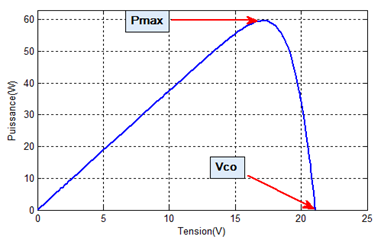
Figure 4 shows the current/voltage characteristic of a cell under constant temperature and lighting conditions: (G=1,000w/m², T=25℃). On this curve, the empty operating point is identified: Vco for I=0A and the shortcircuit operating point: Isc for U=0V, and Figure 5 shows the power characteristic as a function of the voltage. This curve passes through a maximum power (Pmax) at this corresponding power, a voltage Vpm and a current Ipm which can be seen on the curve (I=f (V)).
Figure 4. Characteristic I=f (V)
Figure 5. Characteristic P=f (V)
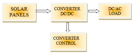
Under these conditions, for the GPV to provide its maximum power, an adaptation is made by interposing a DC/DC power converter between the GPV and the load (see Figure 6, which shows the structure of PV system) [5]. This DC/DC quadrupole is fitted with the MPPT control which in turn has the P&O algorithm to track the MPP in order to deliver only the maximum power to the load.
Photovoltaic generators have a random electrical production directly dependent on weather conditions. Thus, the optimal dimensioning and utilization of the energy produced by these generators requires the use of appropriate management methods.
Figure 6. Diagram of a PV system
Figure 7. Algorithm of the (P&O)
The improvement of the efficiency of the photovoltaic system requires the maximization of the power of the PV generator, which makes it possible to establish the appropriate control in order to derive the maximum power from these generators. The MPPT control makes it possible to find the optimum operating point of the photovoltaic module in stable weather and load conditions. This is based on the automatic variation of the duty cycle α of the signal controlling the energy converter to an appropriate value so as to maximize the output power of the module [6].
In order to extract the maximum power of a solar panel, one can rely on the (P&O) algorithm which is the most commonly used in practice due to its simplicity and ease of implementation and requires only the measurement of V and IPV. However, it has limitations that reduce its MPPT effectiveness. One of them occurs when the amount of sunlight decreases, the P=f(V) curve flattens, and this makes it difficult to discern the location of the MPP, due to the small change in power compared to the voltage disturbance. The other fundamental disadvantage of P&O is that it cannot determine when it has actually reached the MPP. Instead, it oscillates around the MPP, changing the sign of the disturbance after each measurement. Figure 7 shows the flow chart of the P&O algorithm.
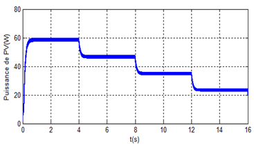
We have tested the performance of the algorithm by simulation. The results are shown in Figures 8 and 9. It represents respectively the variation of the illumination and the power delivered by the PV system. During this simulation, the system is subjected to a change in brightness of [1000, 800, 1000] W/m2 at times (0, 4, 8s) under the effect of a constant temperature. MPPT technique follows the variation of the irradiation with a rather remarkable rapidity.
Figure 8. Variation of the irradiance with time
Figure 9. Power of PV in function of time T=25℃
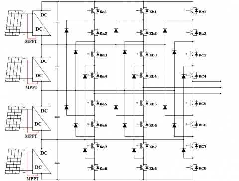
If we consider each of the phases of the three-phase inverter NPC with 5 levels, we find that it is composed of eight switches with unidirectional control in voltage and bidirectional in current. These are classic combinations of a transistor and an anti-parallel diode and six hold diodes connected along the DC bus [7-9].
The inverter is fed by a continuous source E; it has four equal capacitors to give four distinct equal sources (E/4). The three-phase structure of the NPC inverter with 5 levels is shown in Figure 10.
Figure 10. Structure of a five-level NPC inverter
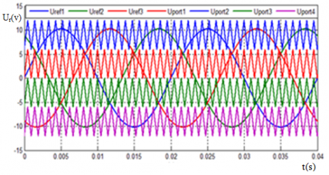
The classic sinusoidal technique with a single triangular signal is not suitable for inverters with levels greater than three, because it does not make it possible to generate all the necessary control signals, which leads to the use of a multi-triangular sinusoidal modulation.
To control the five-level inverter by pulse-width modulation (PWM), a strategy is used to generate the most sinusoidal voltage possible, where the four-carrier triangular sinusoidal drive whose algorithm is defined in the Table 2. The Figure 11 below shows the four triangular sinusoidal control signal carriers.
The phase-to-neutral voltage can assume (the voltage between the arm of the inverter and point 0). The possible states of a single switch arm are 25=32 states which can be represented by a quadruplet of 0 and 1. Table 3 presents the excitation table associated with this complementary command. Only the following five states are possible:
Figure 11. Four carriers triangular sinusoidal control signals
Table 2. Control algorithm of the five-level inverter
|
Test |
UKM |
|
Ur<Up1 |
0 |
|
Ur≥Up1 |
E/2 |
|
Ur<Up2 |
0 |
|
Ur≥Up2 |
E/4 |
|
Ur<Up3 |
0 |
|
Ur≥Up3 |
0 |
|
Ur<Up4 |
-E/2 |
|
Ur≥Up4 |
-E/4 |
First configuration 11110000: Ka1, Ka2, Ka3 and Ka4 are conductive and Ka5, Ka6, Ka7 and Ka8 are blocking, the phase-to-neutral voltage value Uao is given by the following equation: Uao=E/2. The negative sequence voltage applied to the terminals of the blocked switches is: Uka5=Uka6=Uka7=Uka8= E/4.
Second configuration (01111000): Ka2, Ka3, Ka4 and Ka5 are conductive and Ka6, Ka7, Ka8 and Ka1 are blocking, the phase-to-neutral voltage value is Uao=E/4. The negative sequence voltage applied to the terminals of the blocked switches is: Uka1 = Uka6 = Uka7 = Uka8 = +E/4.
Third configuration (00111100): Ka3, Ka4, Ka5 and Ka6 are conducting and Ka7, Ka8, Ka1 and Ka2 are blocking. The phase-to-neutral voltage value Uao is given by the following equation: Uao=0. The negative sequence voltage applied to the terminals of the blocked switches is: Uka1=Uka2=Uka7=Uka8=E/4.
Fourth configuration (00011110): Ka4, Ka5, Ka6 and Ka7 are conducting and Ka8, Ka1, Ka2 and Ka3 are blocking. The phase-to-neutral voltage value is Uao=-E/4. The reverse voltage applied to the terminals of blocked switches is: Uka1=Uka2=Uka3=Uka8=+E/4.
Fifth configuration 00001111: Ka5, Ka6, Ka7 and Ka8 are conducting and Ka1, Ka2, Ka3 et Ka4 are blocking. The phase-to-neutral voltage value is Uao=-E/2. The reverse voltage applied to the terminals of blocked switches is: Uka1=Uka2=Uka3=Uka4=E/4.
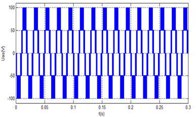
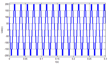
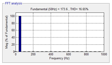
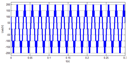
Figures 12 and 13 respectively show the voltage of phase A and the harmonic distortions obtained with it. Note that the results give the following voltage levels: E/2, E/4, 0, -E/4,-E/2. The voltage obtained between phases A and B is represented by Figure 14 and its harmonic distortions are shown in Figure 15.
Table 3. Output voltages of the 5 levels NPC inverter with the states of the switches
|
Sequences |
1 |
2 |
3 |
4 |
5 |
|
|
Switches |
Ki1 |
1 |
0 |
0 |
0 |
0 |
|
Ki1 |
1 |
1 |
0 |
0 |
0 |
|
|
Ki1 |
1 |
1 |
1 |
0 |
0 |
|
|
Ki1 |
1 |
1 |
1 |
1 |
0 |
|
|
Ki1 |
0 |
1 |
1 |
1 |
1 |
|
|
Ki1 |
0 |
0 |
1 |
1 |
1 |
|
|
Ki1 |
0 |
0 |
0 |
1 |
1 |
|
|
Ki1 |
0 |
0 |
0 |
0 |
1 |
|
|
Output Voltage |
Ui0 |
+E/2 |
+E/4 |
0 |
-E/4 |
-E/2 |
Figure 12. Simulation single voltage Uao of the 5 levels NPC inverter with PWM
Figure 13. Simulation spectral analysis Uao of the 5 levels NPC inverter with PWM
Figure 14. Simulation of compound voltage Uab for 5-level NPC inverter with PWM
Figure 15. Simulation of spectral analysis Uab for 5-level NPC inverter with PWM
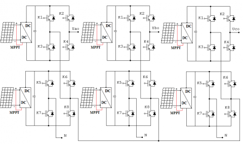
The Figure 16 shows the structure of a multi-level converter based on the series connection of single-phase inverters (H-bridge, or partial cell). The structure of a five-stage inverter arm of H-bridge cascade type is the cascade combination of two conventional single-phase inverters in full bridge [10-12], so that the output voltage of the inverter obtained is the sum of output voltages of the two conventional inverters.The five possible states or switching sequences are summarized in Table 4.
Figure 16. Three-phase structure of a five-level H-bridge cascade inverter
Table 4. Output voltage of the 5 stage inverter in H-bridgeaccording to the states of the switches
|
Switches |
K1 |
1 |
1 |
0 |
0 |
0 |
|
K2 |
0 |
0 |
1 |
1 |
1 |
|
|
K3 |
0 |
0 |
0 |
1 |
1 |
|
|
K4 |
1 |
1 |
1 |
0 |
0 |
|
|
K5 |
1 |
0 |
0 |
0 |
0 |
|
|
K6 |
0 |
1 |
1 |
1 |
1 |
|
|
K7 |
0 |
0 |
0 |
0 |
1 |
|
|
K8 |
1 |
1 |
1 |
1 |
0 |
|
|
Output voltage |
Ua0 |
2E |
E |
0 |
-E |
-2E |
Respectively, Figure 17 and 18 present the phase A voltage and its harmonic distortions. Note that the results give the following voltage levels: E/2, E/4, 0, -E/4, -E/2. The voltage between phase A and phase B obtained at the output of the inverter is shown in Figure 19 and Figure 20 presents the harmonic distortions produced from this compound voltage of phase.
Figure 17. Simulation Single voltage Uao of the 5-level inverter in (H-bridge)
Figure 18. Simulation of the spectral analysis Uao of the 5 level inverter in H-bridge
Figure 19. Simulation of the compound voltage Uab of 5 level inverter in H-bridge
Figure 20. Simulation of the spectral analysis Uao of the 5 level inverter in H-bridge
Our results presented in Table 5, have clearly highlighted the supremacy of the multi-level inverter with an NPC structure, for its considerable reduction of the THD, therefore improving the quality of energy. On the other hand, with the H-bridge structure, the same number of levels can be obtained with the same number of switches without holding diodes or floating capacitors. The use of multi-level inverters in the H-Bridge presents a solution with minimal components and simpler manufacturing.
Table 5. Results obtained from the two various structures
|
Number of level |
5 level |
|
|
Topology |
NPC |
H-Bridge |
|
Number of IGBTs |
24 |
24 |
|
Number of diodes |
18 |
0 |
|
Number of capacitors |
16 |
0 |
|
THD UAO (%) |
26,21 |
33,49 |
|
THD UAB (%) |
16,65 |
28,75 |
In this article, we introduced two types of multilevel inverters, H-bridge cascade and NPC structures. These two structures are most often used in the connection to the electrical grid of the generators of PV systems. We modeled respectively the 5-level NPC and H-bridge inverters with the triangular sinusoidal PWM control strategy, which allows the simulation of the grid-connected photovoltaic generator system. The spectral study of the two previous topologies showed the superiority of the NPC converter. However, we have demonstrated that with the structure of the H-bridge, the same number of levels can be obtained with the same number of switches and without holding diodes or floating capacitors.
However, for each additional pair of levels, an additional voltage source is required. Multi-level inverters allow connecting simultaneously several systems from GPV to electrical networks with a possibility to work at high power while improving the quality of delivered energy.
The use of multi-level inverters with an NPC structure reduces the THD, which allows us to use more limited filtering. However, the use of multi-level inverters in the H Bridge presents a solution with a minimum of components and simpler manufacturing.
[1] Park, H., Kim, Y.J., Kim, H. (2016). PV cell model by single-diode electrical equivalent circuit. Journal of Electrical Engineering and Technology, 11(5): 1323-1331. https://doi.org/10.5370/JEET.2016.11.5.1323
[2] Chaibi, Y., Salhi, M., El-Jouni, A., Essadki, A. (2018). A new method to extract the equivalent circuit parameters of a photovoltaic panel. Solar Energy, 163: 376-386. https://doi.org/10.1016/j.solener.2018.02.017
[3] Sesa, E., Vaughan, B., Feron, K., Bilen, C., Zhou, X., Belcher, W., Dastoor, P. (2018). A building-block approach to the development of an equivalent circuit model for organic photovoltaic cells. Organic Electronics, 58: 207-215. https://doi.org/10.1016/j.orgel.2018.04.019
[4] Gupta, K.K., Jain, S. (2012). Topology for multilevel inverters to attain maximum number of levels from given DC sources. IET Power Electronics, 5(4): 435-446. https://doi.org/10.1049/iet-pel.2011.0178
[5] Soufyane Benyoucef, A., Chouder, A., Kara, K., Silvestre, S. (2015). Artificial bee colony based algorithm for maximum power point tracking (MPPT) for PV systems operating under partial shaded conditions. Applied Soft Computing, 32: 38-48. https://doi.org/10.1016/j.asoc.2015.03.047
[6] De Brito, M.A.G., Galotto, L., Sampaio, L.P., e Melo, G.D.A., Canesin, C.A. (2012). Evaluation of the main MPPT techniques for photovoltaic applications. IEEE Transactions on Industrial Electronics, 60(3): 1156-1167. https://doi.org/10.1109/TIE.2012.2198036
[7] Babaie, A., Karami, B., Abrishamifar, A. (2016). Improved equations of switching loss and conduction loss in SPWM multilevel inverters. In 2016 7th Power Electronics and Drive Systems Technologies Conference (PEDSTC), pp. 559-564. https://doi.org/10.1109/PEDSTC.2016.7556921
[8] Ramu, J., Parkash, S., Srinivasu, K., Ram, R., Prasad, M., Hussain, M. (2012). Comparison between symmetrical and asymmetrical single phase seven level cascaded h-bridge multilevel inverter with PWM topology. International Journal of Multidisciplinary Sciences and Engineering, 3(4): 16-20.
[9] Patel, A., Joshi, S., Chandwani, H., Patel, V., Patel, K. (2010). Estimation of junction temperature and power loss of IGBT used in VVVF inverter using numerical solution from data sheet parameter. International Journal of Computer Communication and Informatics System (IJCCIS), 2(1).
[10] Muñoz-Cruzado-Alba, J., Rojas, C.A., Kouro, S., Galván Díez, E. (2016). Power production losses study by frequency regulation in weak-grid-connected utility-scale photovoltaic plants. Energies, 9(5): 317. https://doi.org/10.3390/en9050317
[11] Lee, T., Bu, H., Cho, Y. (2019). Hybrid PWM strategy for power efficiency improvement of 5-Level TNPC inverter and current distortion compensation method. Electronics, 8(1): 76. https://doi.org/10.3390/electronics8010076
[12] Chub, A., Vinnikov, D., Blaabjerg, F., Peng, F.Z. (2015). A review of galvanically isolated impedance-source DC–DC converters. IEEE Transactions on Power Electronics, 31(4): 2808-2828. https://doi.org/10.1109/TPEL.2015.2453128