Moussa Attia* | Mohcene Bechouat | Moussa Sedraoui | Zoubir Aoulmi
© 2022 IIETA. This article is published by IIETA and is licensed under the CC BY 4.0 license (http://creativecommons.org/licenses/by/4.0/).
OPEN ACCESS
In this paper, a steady-state output power oscillation problem is overcome using the indirect control mode based-Perturb and Observe (P&O) implementation algorithm. This can be ensured through controlling the duty cycle input of the DC-DC boost converter using the proposed Linear Quadratic Regulator (LQR) controller. Their parameters are optimized using the Grasshopper Optimization Algorithm (GOA) where a good tracking behavior of a desired Maximum Power Point (MPP) can be guaranteed for various sudden changes in weather conditions such as absolute temperature and solar irradiance. The desired performances and robustness of the closed-loop system can be achieved by the two following stages. In the first stage, the standard P&O algorithm based-direct control mode generates a reference current perturbation using both existing electrical power and measured PV current. Accordingly, a current error perturbation is provided through the discrepancy between reference and measured currents. In the second stage, the previous current error provided in the inner control-loop is mitigated as much as possible using the stabilized LQR controller. The current control-loop problem is addressed with a detailed analysis technique of averaging and linearization, in which the linearization of actual PV-boost converter system around the desired MPP allows determining the corresponding linear plant-model. This leads to well optimize the LQR controller parameters. The performance and robustness provided by the P&O algorithm based-indirect duty cycle control are shown for sudden changes in solar irradiance and absolute temperature as well as in a wide variation of the resistive load.
PV panel, DC-DC boost converter, maximum power point tracking MPPT controller, grasshopper optimization algorithm GOA
In general, solar energy is one of the most promising renewable sources needed largely in industrial and domestic applications. The electricity production based-solar energy is usually ensured through PV panel which manufactured from parallel and series connections of several solar cells. Indeed, the solar cell converts the energy of sunlight photons into electricity by means of the photoelectric phenomenon existing in certain semiconductor materials such as silicon and selenium [1].
In real-world applications, the main concern of most renewable energy engineers is how to ensure the maximal electrical power from any PV panels. The Maximum Power Point Tracking MPPT is one of the most commonly used control strategies to ensure a good MPP tracking behavior of the PV panel, regardless of sudden changes in weather conditions. Indeed, the MPP follow-up issue has been addressed in many literatures [2]. Among them, P&O-MPPT is the widely algorithm used to regulate the duty cycle of the DC-DC boost converter. This last is commonly used as an interface between the PV panel and the external load. Moreover, P&O-MPPT algorithm can be applied on the closed-loop system based PV panel, DC-DC boost converter and external load using either control modes: direct duty cycle control mode or indirect duty cycle control based-stabilized controller [2, 3]. This study focused only on the second previous control mode, in which the way of designing the stabilized controller presents the main contribution of this paper.
In general, the indirect control mode of the duty cycle via a stabilized controller has the capacity to provide a better trade-off between performances and robustness compared by the direct duty cycle control mode. This superiority depends heavily on the proper choice of the synthesis step of the stabilized controller. This controller can be used to regulate either outputs PV voltage or PV current at the load, to control the power flow in grid-connected systems and mainly to well follow the desired MPP [3]. Indeed, the indirect control mode based on P&O-MPPT algorithm has recently attracted several scholars [4-9].
Among them, Villalva et al. [4] proposed two small-signal models for the KC200GT solar array. The first model is used for the current regulation wherein the second one is used for the voltage regulation. The voltage control loop is ensured using the Proportional- Integral (PI) controller and the closed-loop performances are evaluated under several climatic conditions. In the same direction, Kollimalla and Mishra [5] proposed a new adaptive P&O-MPPT algorithm based-reference current perturbation for a PV panel of type Solarex-MSX60. The current control loop is ensured by the PI controller and the given experimental results show that the proposed algorithm gives faster response than the conventional P&O-MPPT algorithm for sudden changes in the irradiance. Furthermore, Harrag and Messalti [6] generated a variable step-size from P&O-MPPT algorithm using the genetic algorithm (GA). The Proportional-Integral-Derivative (PID) controller is included for the voltage regulation, providing thus a fast PMM tracking behavior in the presence of several weather conditions. In addition, Althobaiti et al. [7] proposed a small-signal model for the voltage regulation. The control loop is performed using either stabilized controllers: The Proportional controller equipped with the low-pass filter or the PI controller synthesized by the root locus based-second Ziegler-Nichols method. The simulation results show that the proposed algorithm offers better stability characteristics over those provided by the conventional P&O-MPPT algorithm. Lasheen, et al. [8] proposed an adaptive reference voltage-based MPPT technique for PV panel, which is exposed to a radiation profile with fast rate of change. The boost mathematical model is firstly designed and its duty cycle input is then controlled using the stabilized PI controller. The controller parameters are determined by a trial-and-error approach where the desired MPP is captured, even during a rapid variation of the solar irradiance. Recently, Raiker et al. [9] introduced a momentum term in the conventional P&O-MPPT algorithm to accelerate tracking and to reduce oscillations. The inner current control loop of the P&O-MPPT scheme is ensured by a two Degree-of-Freedom (2-DOF) controller. Accordingly, the corresponding post-compensator is introduced to enhance the robustness of the closed loop system against the model uncertainties wherein the corresponding pre-compensator is introduced to enhance the closed-loop performances.
According to all previous works, this paper addresses the control problem of extracting the maximum electrical power of PV system where the adequate reference PV current perturbation is generated by the standard P&O algorithm and the adequate duty cycle perturbation is then provided by the stabilized LQR controller. This last is synthesized through the small-signal model which describing the linear behavior of the DC-DC boost converter around the desired MPP. This paper is organized as follows: section 2 is reserved for the modeling step of the PV panel using the equivalent electrical circuit based-single diode. In section 3, the small-signal model describing the linear behavior of the DC-DC boost converter is detailed. The step response and the frequency response based- Bode diagram of this model are illustrated in section 4. The standard P&O algorithm and the improved-LQR are detailed in section 5, then, simulation results are presented in section 6. Finally, the whole of this paper is achieved by a conclusion.
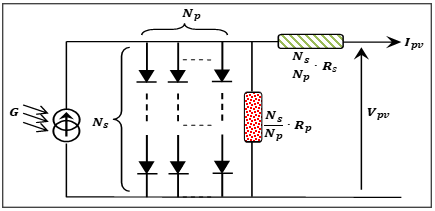
In general, the actual PV cell behavior can be described by an equivalent electrical circuit based-single [6, 10]. Accordingly, for the PV panel arranged in $N_{p}$ parallel strings and $N_{s}$ series cells, the corresponding equivalent electrical circuit can be presented in Figure 1. It consists of $N_{p}$ photocurrent sources, $\frac{N_{s}}{N_{p}}$ parallel resistors representing a leakage current, $N_{p} \times N_{s}$ diodes, and $\frac{N_{s}}{N_{p}}$ series resistors describing an internal resistance to the current flow [5, 11].
Figure 1. Equivalent electrical circuit of the PV panel model
According to Figure 1, the predicted PV current model is given by [11, 12]:
$I_{p v}=N_{p} \cdot I_{p h}-N_{p} \cdot I_{D}-\frac{N_{p}}{N_{s} \cdot N_{c} \cdot R_{p}} \cdot V_{p v}-\frac{R_{s}}{R_{p}} \cdot I_{p v}$ (1)
where, $I_{D}$ and $I_{0}$ are respectively defined by:
$I_{D}=I_{0}(-1+e^{\frac{q}{n \cdot K \cdot T} \cdot\left(\frac{1}{N_{c} \cdot N_{S}} \cdot V_{p v}+\frac{R_{S}}{N_{p}} \cdot I_{p v}\right)})$ (2)
$I_{0}=\sqrt[n]{\left(\frac{T}{T_{s t c}}\right)^{3}} \cdot \frac{I_{s c}}{-1+e^{\frac{q}{n \cdot K \cdot T} \cdot\left(\frac{1}{N_{c} \cdot N_{s}} \cdot V_{p v}+\frac{R_{s}}{N p} \cdot I_{p v}\right)}} \quad \cdot e^{\frac{q \cdot v_{g}}{n} \cdot\left(\frac{1}{\frac{1}{T}-\frac{1}{T_{s t c}}}\right)}$ (3)
Table 1. Data sheet of the PV panel
|
Parameter |
Meaning parameter |
Value |
|
G |
Current solar irradiance |
- |
|
T |
Current absolute temperature |
- |
|
Ipv |
Output current predicted by the PV panel model |
A |
|
Vpv |
Output voltage predicted by the PV panel model |
V |
|
Iph |
Generated photo-current |
A |
|
Isc |
short-circuit current |
3.80 A |
|
ID |
Current passing through the diode D |
- |
|
I0 |
Reverse saturation current of the diode D |
- |
|
n |
Ideality factor of the diode D |
1.2 |
|
Rs |
Series resistor |
0.0018 Ω |
|
Rp |
Shunt resistor |
150 Ω |
|
Nc |
Number of the PV cell |
36 |
|
Ns |
Number of solar cells connected in series |
1 |
|
Np |
Number of solar cells connected in parallel |
1 |
|
k |
Boltzmann’s constant |
1.6×10⁻²³ J∙K-1 |
|
T |
Temperature of solar cells |
K |
|
q |
Electron charge |
1.6×10⁻¹⁹ C |
|
Vg |
Band-gap energy of the semiconductor |
2.2 e-V |
|
GSTC |
Nominal solar irradiance |
1000 W/m2 |
|
TSTC |
Nominal absolute Temperature |
298.15K |
Table 1 summarizes the data sheet of the PV panel and their specification at the Standard Test Condition (STC) [11, 13].
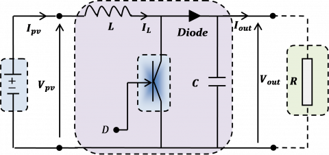
The DC-DC boost converter is usually operated in Continuous Conduction Mode (CCM), providing thus a pure nonlinear behavior. The corresponding small-signal model which associating its duty cycle perturbation input with the PV current perturbation output should be determined using the average variable method described in Refs. [5, 14]. The equivalent electrical circuit describes the linear behavior of the DC-DC boost converter around the desired can be shown in Figure 2 [15, 16].
Figure 2. Equivalent electrical circuit of DC-DC boost converter
According to Figure 2, the following equations used to approximate the DC-DC boost converter model are given by [5, 6]:
$\frac{d}{d t} I_{p v}=\frac{1}{L} \cdot V_{p v}-\frac{1-D}{L} \cdot V_{\text {out }}$
$\frac{d}{d t} V_{o u t}=\frac{1-D}{C} \cdot I_{p v}-\frac{1}{R \cdot C} \cdot V_{o u t}$ (4)
Knowing that, for constant level of the solar irradiance and high inertia of the PV panel in function of the absolute temperature variation, the output current Ipv can be defined as follow [5, 6]:
$I_{p v}=-\frac{1}{R_{M P P}} \cdot V_{p v}$ (5)
where, RMPP denotes the total resistor of the PV panel given at MPP. Furthermore, by substituting Eq. (5) in Eq. (4), the state-space representation of the DC-DC Boost converter model is given by Eqns. (5) and (6):
$\frac{d}{d t} I_{p v}=-\frac{R_{M P P}}{L} \cdot I_{p v}-\frac{1-D}{L} \cdot V_{o u t}$
$\frac{d}{d t} V_{o u t}=\frac{1-D}{C} \cdot I_{p v}-\frac{1}{R \cdot C} \cdot V_{o u t}$ (6)
According to the small-signal principal, the relationships which associate the state variables $I_{p v}, V_{\text {out }}$ and $D$ at MPP with respectively their small perturbations $\delta I_{p v}, \delta V_{\text {out }}$ and $\delta D$ are defined by $I_{p v}=I_{p v_{M P P}}+\delta I_{p v}, V_{o u t}=V_{o u t}^{M P P}+\delta V_{o u t}$ and $D=D_{M P P}+\delta D$. Moreover, the output voltage $V_{\text {out }}$ of the DC-DC boost converter is determined for the resistive load $R$, assuming a loss less converter, i.e., $P_{\text {out }}=P_{p v}$. Therefore, the output voltage $V_{o u t_{M P P}} \quad $ and its corresponding duty cycle $D_{M P P}$ , when the steady-state quantities are removed and the two second-order perturbation quantities $\delta D$. $\delta V_{\text {out }}$ and $\delta D \cdot \delta I_{p v}$ are neglected, the linear state-space representation of the small-signal model of the DC-DC boost converter is given in [6, 16] by:
$\frac{d}{d t} \delta I_{p v}=-\frac{R_{M P P}}{L} \cdot \delta I_{p v}-\left(\frac{1-D_{M P P}}{L} \quad \right) \cdot \delta V_{\text {out }}+\frac{V_{\text {out }_{M P P}}}{L} \cdot \delta D$
$\frac{d}{d t} \delta V_{\text {out }}=\left(\frac{1-D_{M P P}}{C} \quad \right) \cdot \delta I_{p v}-\frac{1}{R \cdot C} \cdot \delta V_{o u t}-\frac{I_{p v_{M P P}}}{C} \cdot \delta D$ (7)
The Eq. (10) can be reformed in linear state-space equations which are:
$\left\{\begin{array}{l}\dot{x}=A \cdot x+B \cdot u \\ y=C \cdot x+D \cdot u\end{array}\right.$ (8)
where, x is the state, u is the control input, A, B, C and D are state-space matrices. For the system, the state and output are defined:
$\left\{\begin{array}{c}x=\left[\begin{array}{ll}\delta I_{p v} \quad \delta V_{o u t}\end{array}\right] \\ y=\delta I_{p v}\end{array}\right.$ (9)
Based on Eq. (7) to Eq. (9), the A, B, C and D matrices are defined:
$\left\{\begin{array}{c}A=\left[\begin{array}{c}-\frac{R_{M P P}}{L}-\left(\frac{1-D_{M P P}}{L}\right) \\ \frac{1-D_{M P P}}{C}-\frac{1}{R \cdot C}\end{array}\right] \\ B=\left[\begin{array}{l}\frac{V_{o u t}}{L P P} \\ \frac{I_{p v_{M P P}}}{C}\end{array}\right] \\ C=\left[\begin{array}{ll}1 & 0\end{array}\right] \\ D=0\end{array}\right.$ (10)
Also, the s-domain of Eq. (7) can be involved the following transfer function F(s) which associating the current perturbation output $\delta I_{p v}$ with the duty cycle perturbation input $\delta D$. It yields the following transfer function:
$F(s)=k_{0} \cdot \frac{s+b_{0}}{s^{2}+a_{1} \cdot s+a_{0}}$ (11)
where, $k_{0}=\frac{V_{o u t}}{L P P}$, $b_{0}=\frac{1}{R \cdot C}\left(1+\cdot \frac{R \cdot\left(1-D_{M P P} \quad \right) \cdot I_{p v_{M P P}}}{V_{o u t}} \quad \right)$, $a_{1}=\frac{1}{R \cdot C}$ and $a_{0}=\frac{1-D_{M P P}}{L \cdot C}$.
The parameters of the DC-DC boost converter model as well as the MPP measurements are summarized in Table 2 [12, 13].
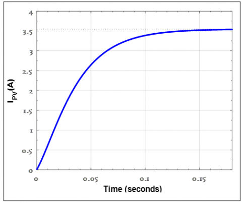
Figure 3 shows the step response provided when the transfer function of the DC-DC boost converter model is excited by the duty cycle input $D_{M P P}=0.5116$ for the resistive load $R=20 \Omega$.
According to Figure 3, it is easy to see that the output current response converges to the MPP current $I_{o u t_{M P P}} \quad =3.56 \mathrm{~A}$ in the steady-state. This confirms the validity of the given small-signal model to synthesize the stabilized LQR controller.
Table 2. Meaning and values of the DC-DC boost converter model and MPP measurements
|
Parameters |
Values |
|
Input inductor |
350 mH |
|
Capacitor C |
560 μF |
|
Duty cycle generated at $M P P\left(D_{M P P}\right)$ |
0.5116 |
|
Output voltage provided at $M P P\left(V_{o u t_{M P P}} \quad \right)$ |
17.00 V |
|
Output current provided at $\operatorname{MPP}\left(I_{\text {out }_{M P P}} \quad \right)$ |
3.56 A |
Figure 3. Time response of the small-signal model given at duty cycle input $D_{M P P}$
In addition, Figure 4 shows the Bode plot of the open loop system of the reference current control given by the conjunction of the small-signal model F(s) with the proportional controller $K_{P}=1$ to adjust the duty cycle ration for the same previous resistive load $R=20 \Omega$.
Figure 4. Bode plot of the small-signal DC-DC boost converter model
According to Figure 4, it is easy to confirm that the closed-loop system is still stable, which requires an optimal controller to improve their performances.
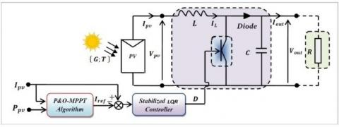
Once the reference current perturbation is generated by the aforementioned algorithm (see Figure 6), the inner current control loop based- small-signal model including the desired stabilized LQR is illustrated in Figure 5 [6, 17].
Figure 5. P&O-MPPT scheme equipped with a stabilized LQR current controller
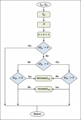
Figure 6. Flow chart of the P&O-MPPT algorithm to provide the reference PV current
4.1 P&O-MPPT algorithm
In this paper, the main goal of the P&O algorithm is to generate the reference current perturbation $\delta I_{r e f}$ from the both output power measurement as well as the output current measurement. Figure 6 gives the Flow chart of the P&O-MPPT algorithm [4-6].
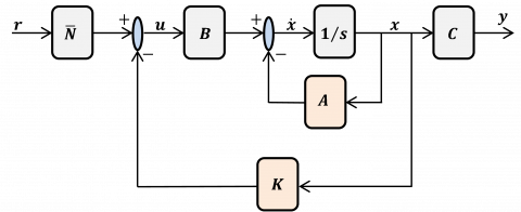
4.2 Conventional LQR strategy
LQR is a full state feedback optimal controller which minimizes the quadratic cost function based on states of system and input vectors. While designing LQR controller is shown in Figure 7.
Figure 7. Full state feedback control design
Given that the equations of motion of the system can be described in Eq. (8). Where A and Bare the state and input system matrices, respectively, the LQR algorithm computes a control law u such that the performance criterion or cost function is minimize:
$J=\int_{0}^{\infty}\left(x^{T} Q x+u^{T} R u\right) d t$ (12)
Q and R are positive-definite (or positive-semi definite) Hermitian or real symmetric matrices and are known as weighting matrices. Theirs design hold the penalties on the deviations of state variables from their set point and the control actions, respectively. When an element of Q is increased, therefore, the cost function increases the penalty associated with any deviations from the desired set point of that state variable, and thus the specific control gain will be larger. When the values of the R matrix are increased, a larger penalty is applied to the aggressiveness of the control action, and the control gains are uniformly decreased. Notes here, that in our case Q and R are given by:
$\left\{\begin{array}{l}Q=\left[\begin{array}{cc}q_{1} & 0 \\ 0 & q_{2}\end{array}\right] \\ R=\text { constant }\end{array}\right.$ (13)
The feedback law that minimizes the cost function is given by:
$u=-k \cdot x$ (14)
where, the value of k matrix is found by:
$k=R^{-1} \cdot B^{T} \cdot P$ (15)
The matrix P is found by solving the continuous time algebraic Riccati equation given below:
$0=A^{T} \cdot P+B \cdot A-P \cdot B \cdot R^{-1} \cdot P^{T} \cdot B+Q$ (16)
4.3 Improved LQR strategy
In this study, the main contribution lies in the selection of the two optimal matrices Q and R involved in to calculate the k matrix. The corresponding bounded optimization problem includes the fitness function f(X), expressed as the MSE criterion. It consists of the sum of the squared error e, produced by the simultaneous tracking of the reference power in STC which is PSTC and the measured power $P_{\text {measured }}$. Accordingly, the optimization problem can be expressed by:
$\min _{X_{\min } \leq X \leq X_{\max }} \quad f(X)=\min _{X_{\min } \leq X_{\max }}\left\{\frac{1}{N T} \sum_{i=1}^{N} e^{2}(X)\right\}$ (17)
where, the tracking error e is defined by:
$e(X)=P_{\text {measured }}(X)-P_{S T C}, X=\left(q_{1}, q_{2}, R\right)^{T}$ denotes the design vector to be optimized where their components are constrained by $0 \leq X \leq \infty, N$ and $T$ denote the total number of samples and the sampling time.
The GOA algorithm is implemented in a classical LQR strategy to focus on finding the optimal Q and R during the tracking process of the optimal power. These optimal values lead to finding the feasible optimal control. The optimization process by the GOA algorithm is carried out as follows:
The GOA algorithm uses a mimic the swarming behavior of grasshoppers $n_{p} \in \mathbb{N}$ to know in search of the sub-optimal solution $X^{*} \in \mathbb{N}^{m \times 1}$ which minimizes the objective function, called $f(X) \in \mathbb{R}$.The position and the social communication of grasshopper vectors $i^{\text {th }}$ are given respectively by: $X_{i}=$ $\left(X_{i, 1}, X_{i, 2}, \ldots, X_{i, m}\right)^{T}$ and $S_{i}=\left(S_{i, 1}, S_{i, 2}, \ldots, S_{i, m}\right)^{T}$. They are determined by the following expressions [18-21]:
$X_{i}^{d}=c\left(\sum_{j=1}^{m} c \frac{X_{\min }^{d}-X_{\max }^{d}}{2} S_{i}^{d}\right)+X_{\text {best }}^{d}$ (18)
where, c is a coefficient decreases the comfort region equivalent the number of generation is computed by:
$c=1-$ current generation $\times\frac{1-0.00001}{\text { largest number of generation }}$ (19)
And d is the number of iterations previously provided by the user. the Si is computed by the following expression:
$S_{i}^{d}=s\left(d_{i j}^{d}\right) \widehat{d_{i j}}$ (20)
where, $s$ is a mathematical function to determine the power of social organizations related by the power of attraction $f$ and the attractive $l, d_{i j}^{d}$ represents the distance value between the $i_{t h}$ and the $j_{t h}$ grasshopper, $\widehat{d_{i j}}$ represents a block vector from the $i_{t h}$ grasshopper to the $j_{t h}$ grasshopper as shown in Eq. (20).
$\left\{\begin{array}{c}s(r)=f e^{\frac{-r}{l}}-e^{-r} \\ d_{i j}^{d}=\left|X_{j}^{d}-X_{i}^{d}\right| \\ \widehat{d_{\imath j}}=\frac{x_{j}-x_{i}}{d_{i j}}\end{array}\right.$ (21)
In summary, the GOA algorithm can consist of the following steps:
Step1: Initialize the Xi grasshopper population considered the lower and upper bounds vectors Xmin and Xmax;
Step2: Evaluate the fitness function for each search agent (solution);
Step3: Determine the best search agent so far $X_{\text {best }}^{i}$;
Step4: Check the stop condition. If it is satisfied, the algorithm then converges to the desired optimal values of matrices Q and R. Otherwise, go to the next step;
Step5: Assign the new values obtained to all agents (updates);
Step6: Go back to step 2.
The output electrical power generated by the PV panel is ensured by two stages. First, the P&O-MPPT algorithm based-direct control mode is applied to generate the reference current perturbation. Afterward, the current control loop is carried-out by Matlab ®/Simulink software using the sampling time $T_{s}=0.1$ milliseconds, the step-size duty cycle $\Delta D=0.01$ and the step-size current $\Delta I=0.01 A$. Moreover, the optimal values obtained are $q_{1}=0.23, q_{2}=0.33$ and $\mathrm{R}=100$ given the feedback gain k=[0.0362 - 0.0428], this is attained by minimizing the MSE value as shown in the fitness plots (Figure 8) provided by the algorithm during the extraction process for 20 execution of the code.
Figure 8. The obtained fitness curve through GOA
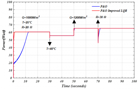
The proposed control strategy is validated at outdoor STC conditions. Indeed, the nominal temperature is increased for 25℃ to 40℃ at the start time t=30 seconds wherein the solar irradiation is being increased from 1000 W/m2 to 1200 W/m2 at the start time t=50 seconds and the load charge value is increased for 20Ω to 30Ω at the start time t=50. Therefore, the MPP tracking behavior provided by the closed-loop system is presented by Figure 9 in term of providing the output electrical power.
Figure 9. Output electrical power of PV system ensured for different conditions
According to Figure 10, it is easy to observe that the closed-loop P&O-MPPT system provides a good tracking behavior of the MPP. This is explained by providing a smooth response of the output electrical power, which is characterized by a fast rise time in transient-state and a less steady-state tracking error. The effect due to the oscillation problem of the output electrical power is well reduced, regardless the sudden change in the solar irradiance.
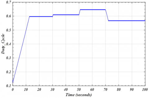
Furthermore, Figure 10 shows the duty cycle response provided by the stabilized LQR controller to drive the switch of DC-DC boost converter which ensuring the previous output electrical power for a sudden change in solar irradiance.
Figure 10. Duty cycle ensured for a sudden change in solar irradiance
A controller synthesis based-small signal model of DC-DC Boost converter has been discussed in this paper. The main goal is to ensure a good MPP tracking behaviour regardless the sudden change in weather conditions, especially in current solar irradiance. The small-signal model is giving from combining the fundamental electrical equations of DC-DC Boost converter with those describing the actual behavior of the PV panel. The desired performances and robustness of the closed-loop P&O-MPPT scheme are ensured through two stages. The aim of the first stage is to generate the adequate reference current perturbation from the provided output current and output electrical power. On the other hand, the goal of the second stage is to mitigate as much as possible the current error perturbation using the stabilized current controller based-LQR structure. The tuning of the LQR parameters is ensured by Grasshopper optimization algorithm GOA where the given simulation results show the effectiveness of the P&O-MPPT algorithm based-indirect duty cycle control mode. It provides a good output electrical power response, characterized by a fast rise time in transient-state and a smooth response in steady-state. These previous properties confirm that the oscillation problem around the desired MPP is well solved which increases the electrical efficiency of the PV panels in the presence of severe climatic conditions.
[1] Fialho, L., Melício, R., Mendes, V.M.F., Estanqueiro, A., Collares-Pereira, M. (2015). PV systems linked to the grid: parameter identification with a heuristic procedure. Sustainable Energy Technologies and Assessments, 10: 29-39. https://doi.org/10.1016/j.seta.2015.01.006
[2] Ismail, M.S., Moghavvemi, M., Mahlia, T.M.I. (2013). Characterization of PV panel and global optimization of its model parameters using genetic algorithm. Energy Conversion and Management, 73: 10-25. https://doi.org/10.1016/j.enconman.2013.03.033
[3] Dolara, A., Leva, S., Manzolini, G. (2015). Comparison of different physical models for PV power output prediction. Solar Energy, 119: 83-99. https://doi.org/10.1016/j.solener.2015.06.017
[4] Villalva, M.G., De Siqueira, T.G., Ruppert, E. (2010). Voltage regulation of photovoltaic arrays: Small-signal analysis and control design. IET Power Electronics, 3(6): 869-880. http://doi.org/10.1049/iet-pel.2008.0344
[5] Kollimalla, S.K. Mishra, M.K. (2014). A novel adaptive P&O MPPT algorithm considering sudden changes in the irradiance. IEEE Transactions on Energy Conversion, 29(3): 602-610. http://doi.org/10.1109/TEC.2014.2320930
[6] Harrag, A. Messalti, S. (2015). Variable step size modified P&O MPPT algorithm using GA-based hybrid offline/online PID controller. Renewable and Sustainable Energy Reviews, 49: 1247-1260. https://doi.org/10.1016/j.rser.2015.05.003
[7] Althobaiti, A., Armstrong, M., Elgendy, M. (2016). Space vector modulation current control of a three-phase PV grid-connected inverter. In 2016 Saudi Arabia Smart Grid (SASG). https://doi.org/10.1109/SASG.2016.7849673
[8] Lasheen, M., Rahman, A.K.A., Abdel-Salam, M., Ookawara, S. (2017). Adaptive reference voltage-based MPPT technique for PV applications. IET Renewable Power Generation, 11(5): 715-722. http//doi.org/10.1049/iet-rpg.2016.0749
[9] Raiker, G.A. Umanand, L. Reddy, B.S. (2018). Perturb and observe with momentum term applied to current referenced boost converter for PV interface. In 2018 IEEE International Conference on Power Electronics, Drives and Energy Systems (PEDES), pp. 1-6. http//doi.org/10.1109/PEDES.2018.8707630
[10] Heydari, E., Varjani, A.Y. (2019). A new variable step-size P&O algorithm with power output and sensorless DPC method for grid-connected PV system. In 2019 10th International Power Electronics, Drive Systems and Technologies Conference (PEDSTC), pp. 545-550. http//doi.org/10.1109/PEDSTC.2019.8697651
[11] Bechouat, M., Younsi, A., Sedraoui, M., Soufi, Y., Yousfi, L., Tabet, I., Touafek, K. (2017). Parameters identification of a photovoltaic module in a thermal system using meta-heuristic optimization methods. International Journal of Energy and Environmental Engineering, 8(4): 331-341. https://doi.org/10.1007/s40095-017-0252-6
[12] Bechouat, M., Sedraoui, M., Feraga, C. E., Aidoud, M., Kahla, S. (2019). Modeling and fuzzy MPPT controller design for photovoltaic module equipped with a closed-loop cooling system. Journal of Electronic Materials, 48(9): 5471-5480. https://doi.org/10.1007/s11664-019-07243-1
[13] Aidoud, M., Feraga, C.E., Bechouat, M., Sedraoui, M., Kahla, S. (2019). Development of photovoltaic cell models using fundamental modeling approaches. Energy Procedia, 162: 263-274. https://doi.org/10.1016/j.egypro.2019.04.028
[14] Dehghanzadeh, A., Farahani, G., Vahedi, H., Al-Haddad, K. (2018). Model predictive control design for DC-DC converters applied to a photovoltaic system. International Journal of Electrical Power & Energy Systems, 103: 537-544. https://doi.org/10.1016/j.ijepes.2018.05.004
[15] Moradi-Shahrbabak, Z., Bakhshai, A., Tabesh, A. (2018). Effect of dc-link capacitor on small signal stability of grid connected PV power plants. In 2018 IEEE 12th International Conference on Compatibility, Power Electronics and Power Engineering (CPE-POWERENG), pp. 1-5. https://doi.org/10.1109/CPE.2018.8372520
[16] Jain, N.K., Jain, K.K., Shah, A.P. (2018). PV panel based micro-inverter using simple boost control topology. In 2018 International Conference on Smart Electric Drives and Power System (ICSEDPS), pp. 1-4. https://doi.org/10.1109/ICSEDPS.2018.8536048
[17] Palanisamy, R., Vijayakumar, K., Venkatachalam, V., Narayanan, R.M., Saravanakumar, D., Saravanan, K. (2019). Simulation of various DC-DC converters for photovoltaic system. International Journal of Electrical and Computer Engineering, 9(2): 917. https://doi.org/10.11591/ijece.v9i2.pp917-925
[18] Abualigah, L., Diabat, A. (2020). A comprehensive survey of the Grasshopper optimization algorithm: results, variants, and applications. Neural Computing and Applications, 32: 15533-15556. https://doi.org/10.1007/s00521-020-04789-8
[19] Dwivedi, S., Vardhan, M., Tripathi, S. (2020). An effect of chaos grasshopper optimization algorithm for protection of network infrastructure. Computer Networks, 176: 107251. https://doi.org/10.1016/j.comnet.2020.107251
[20] Meraihi, Y., Gabis, A.B., Mirjalili, S., Ramdane-Cherif, A. (2021). Grasshopper optimization algorithm: Theory, variants, and applications. IEEE Access, 9: 50001-50024. https://doi.org/10.1109/ACCESS.2021.3067597
[21] Elazab, O.S., Hasanien, H.M., Alsaidan, I., Abdelaziz, A.Y., Muyeen, S.M. (2020). Parameter estimation of three diode photovoltaic model using grasshopper optimization algorithm. Energies, 13(2): 497. https://doi.org/10.3390/en13020497