Youssouf Mini* | Ngac Ky Nguyen | Eric Semail
© 2021 IIETA. This article is published by IIETA and is licensed under the CC BY 4.0 license (http://creativecommons.org/licenses/by/4.0/).
OPEN ACCESS
This paper proposes a sensorless control strategy based on Sliding Mode Observer (SMO) for a Five-phase Interior Permanent Magnet Synchronous Machine (FIPMSM), with a consideration of the third harmonic component. Compared to conventional three-phase machines, the third harmonic of back electromotive force (back-EMF) contains more information. Thus, in this paper, the first and third harmonic components of the five-phase machine are considered to estimate the rotor position which is necessary for the vector control. Simulation results are shown to verify the feasibility and the robustness of the proposed sensorless control strategy.
back-EMF observer, electrical integrated drive, five-phase interior permanent magnet synchronous machine, sensorless control, sliding mode observer
Multiphase machines present some advantages compared to conventional three-phase machines, such as compactness, reliability (operating under the loss of one or more phases), and a reduction in torque ripple at low frequencies even with non-sinusoidal back-EMFs [1, 2]. Recently, multiphase machines have been used in electric drives with the power inverters integrated in machines [3, 4]. The main advantage of this integration is to reduce the global volume and weight of the integrated drives without electromagnetic compatibility phenomena [5, 6]. In fact, this can be an effective solution for applications which require high power density and compactness, such as automotive, marine and aerospace applications [7].
In this context, the replacement of the position encoder mounted at the end of the rotor shaft by a soft position sensor using only already integrated electrical or magnetic sensors becomes interesting. Besides, to improve the precision, which is classically the weakness of the soft sensor, an algorithm taking advantage of the specificities of non-sinusoidal multiphase machines is necessary. In addition, the multiphase machines are appreciated for their tolerance, a soft position sensor added to the position encoder can be also required to bestow redundancy for the angular position used in the vector control.
In the literature, several studies have proposed sensorless control methods for interior permanent magnet synchronous machines (IPMSMs) [8, 9]. Many sensorless control studies are based on observer for three-phase IPMSMs, however only few papers have considered the sensorless control for multi-phase machines [10-12]. Several methods based on the observer, as Model Reference Adaptive System (MRAS) [13], Extended Kalman Filter (EKF) [14], Luenberger Observer (LO) [15] and Sliding Mode Observer (SMO) [16] can be used to perform the sensorless control of electrical machines. Among these methods, SMO will be chosen to achieve the sensorless control of FIPMSMs due to its simple implementation compared to EKF, which results in the calculation burden especially in the case of multiphase machines. Furthermore, in terms of robustness, SMO presents a robust structure against variations of machine parameters (that will be highlighted in this paper) and noise compared to MRAS and LO [17, 18]. Recently, several researches have proved that the chattering phenomenon inherent in the SMO (main disadvantage of SMO who cannot be completely eliminated) can be reduced, by replacing the saturation function by a sigmoid function [18].
In non-sinusoidal multiphase machines, the torque is produced by several harmonics of their back-EMFs and currents. The current regulation requires the rotor position to perform the vector control. Therefore, the estimation of rotor position through each harmonic (that produces a torque) can increase the degree of freedom for the current control loop, and it allows to separately control different harmonics. This can improve the reliability of the control system of FIPMSMs.
Therefore, in this paper, an observer based on sliding mode will be implemented to achieve the sensorless control of considered FIPMSM. The main contribution of this paper is to use not only one harmonic of the FIPMSM as in [10, 17, 19], but also two characteristic harmonics of the five-phase machine to achieve the sensorless control. Therefore, the first and third harmonic components of the back-EMF of the FIPMSM are used to estimate the rotor position, to perform an accurate vector control.
The FIPMSM model in natural frame, without the magnetic saturation and saliency, is given by [20]:
$\vec{v}=R\vec{i}+\left[ L \right]\frac{d\vec{i}}{dt}+\vec{e}$ (1)
with:
$\vec{v}={{\left[ \begin{matrix} {{v}_{1}} & {{v}_{2}} & {{v}_{3}} & {{v}_{4}} & {{v}_{5}} \\\end{matrix} \right]}^{T}}$
$\vec{e}={{\left[ \begin{matrix} {{e}_{1}} & {{e}_{2}} & {{e}_{3}} & {{e}_{4}} & {{e}_{5}} \\\end{matrix} \right]}^{T}}$
$\vec{i}={{\left[ \begin{matrix} {{i}_{1}} & {{i}_{2}} & {{i}_{3}} & {{i}_{4}} & {{i}_{5}} \\\end{matrix} \right]}^{T}}$
$\left[ L \right]=\left[ \begin{matrix} \text{L} & {{M}_{1}} & {{M}_{2}} & {{M}_{2}} & {{M}_{1}} \\ {{M}_{1}} & \text{L} & {{M}_{1}} & {{M}_{2}} & {{M}_{2}} \\ {{M}_{2}} & {{M}_{1}} & \text{L} & {{M}_{1}} & {{M}_{2}} \\ {{M}_{2}} & {{M}_{2}} & {{M}_{1}} & \text{L} & {{M}_{1}} \\ {{M}_{1}} & {{M}_{2}} & {{M}_{2}} & {{M}_{1}} & \text{L} \\\end{matrix} \right]$
where, $\vec{v}$ represents the voltage vector; $\vec{i}$ is the current vector; $\vec{e}$ is the back-EMF vector; R is the stator resistance; L, M1 and M2 represent respectively the stator self-inductance and two mutual inductances.
Applying the Concordia transformation matrix shown in (2), FIPMSM can be decomposed into several fictitious machines that are magnetically decoupled and mechanically coupled (Table 1). Indeed, each fictitious machine is characterized by a quasi-sinusoidal back-EMF [20].
${{\left[ T \right]}^{t}}=\sqrt{\frac{2}{5}}\left[ \begin{matrix} \frac{1}{\sqrt{2}} & \frac{1}{\sqrt{2}} & \frac{1}{\sqrt{2}} & \frac{1}{\sqrt{2}} & \frac{1}{\sqrt{2}} \\ 1 & \cos \left( \alpha \right) & \cos \left( 2\alpha \right) & \cos \left( 3\alpha \right) & \cos \left( 4\alpha \right) \\ 0 & \sin \left( \alpha \right) & \sin \left( 2\alpha \right) & \sin \left( 3\alpha \right) & \sin \left( 4\alpha \right) \\ 1 & \cos \left( 2\alpha \right) & \cos \left( 4\alpha \right) & \cos \left( 6\alpha \right) & \cos \left( 8\alpha \right) \\ 0 & \sin \left( 2\alpha \right) & \sin \left( 4\alpha \right) & \sin \left( 6\alpha \right) & \sin \left( 8\alpha \right) \\\end{matrix} \right]$ (2)
where, $\alpha=\frac{2 \pi}{5}$.
The model of the FIPMSM in the stationary reference frame (α-β) is given by the following equation:
$\left\{ \begin{matrix} {{L}_{p}}\frac{d{{i}_{\alpha 1}}}{dt}=-\begin{matrix} R{{i}_{\alpha 1}}-{{e}_{\alpha 1}}+{{v}_{\alpha 1}} \\\end{matrix} \\ {{L}_{p}}\frac{d{{i}_{\beta 1}}}{dt}=\begin{matrix} -R{{i}_{\beta 1}}-{{e}_{\beta 1}}+{{v}_{\beta 1}} \\\end{matrix} \\ {{L}_{s}}\frac{d{{i}_{\alpha 3}}}{dt}=\begin{matrix} -R{{i}_{\alpha 3}}-{{e}_{\alpha 3}}+{{v}_{\alpha 3}} \\\end{matrix} \\ {{L}_{s}}\frac{d{{i}_{\beta 3}}}{dt}=\begin{matrix} -R{{i}_{\beta 3}}-{{e}_{\beta 3}}+{{v}_{\beta 3}} \\\end{matrix} \\\end{matrix} \right.$ (3)
where, $\vec{\imath}_{\alpha \beta 1}=\left[\begin{array}{ll}i_{\alpha 1} & i_{\beta 1}\end{array}\right]^{T}$ and $\vec{\imath}_{\alpha \beta 3}=\left[\begin{array}{ll}i_{\alpha 3} & i_{\beta 3}\end{array}\right]^{T}$ represent respectively currents of main and secondary fictitious machines. Lp and Ls represent respectively inductances of main and secondary fictitious machines.
Table 1. Fictitious machines and associated harmonics of FIPMSM [20]
|
Fictitious machines |
Associated harmonics |
|
Main machine |
1, 9, 11, …5*k±1 |
|
Secondary machine |
3, 7, 13, …5*k±2 |
|
Homopolar machine |
5, 15, 25, …5*k |
where, k is integer. The homopolar fictitious machine is equal to zero with a star connection.
As the fictitious machines are mechanically coupled, the electromagnetic torque of the FIPMSM can be obtained by the sum of torques provided by all fictitious machines. Therefore, the total torque is calculated as follows:
$\Gamma=\Gamma_{1}+\Gamma_{3}$ (4)
With: $\Gamma_{1}=\frac{\left[\begin{array}{lll}e_{\alpha 1} & e_{\beta 1}\end{array}\right]\left[\begin{array}{ll}i_{\alpha 1} & i_{\beta 1}\end{array}\right]^{T}}{\Omega}$, and $\Gamma_{3}=\frac{\left[\begin{array}{lll}e_{\alpha 3} & e_{\beta 3}\end{array}\right]\left[\begin{array}{ll}i_{\alpha 3} & i_{\beta 3}\end{array}\right]^{T}}{\Omega}$.
where, Γ1 is the torque of the main fictitious machine; Γ3 is the torque of the second fictitious machine; and Ω is the mechanical speed.
The back-EMF in stationary reference frame (α-β) of each fictitious machine is expressed as (only the 1st and 3rd harmonics are considered) [21]:
$\left\{ \begin{array}{*{35}{l}} {{e}_{\alpha 1}}=-{{\psi }_{1}}{{\omega }_{r}}\sin {{\theta }_{p}} \\ {{e}_{\beta 1}}={{\psi }_{1}}{{\omega }_{r}}\cos {{\theta }_{p}} \\ {{e}_{\alpha 3}}=-{{\psi }_{3}}{{\omega }_{r}}\sin {{\theta }_{s}} \\ {{e}_{\beta 3}}=-{{\psi }_{3}}{{\omega }_{r}}\cos {{\theta }_{s}} \\\end{array} \right.$ (5)
where, ψ1 and ψ3 are respectively the first and third harmonic components of permanent magnet flux linkage, ωr is the electrical angular velocity. The angles θp and θs are defined as: θp=pΩt+θ0p and θs=3pΩt+θ0s. Where θ0p and θ0s represent respectively the initial angles of the first and third harmonics of the back-EMF.
To perform accurate vector control, the rotor position and speed information are required to compute the Park transformation in the rotor reference frame. In this context, it can be seen in (5) that the back-EMF signal contains this two information. From (5), it can be noticed that in the case of the non-sinusoidal FIPMSM (where the back-EMF contains the 1st and 3rd harmonic), the rotor position and speed can be estimated through the two fictitious machines (defined by the Concordia matrix (2)). Thus, an observer based on Sliding Mode will be designed, in order to estimate with high accuracy, the back- EMF signals necessary to extract the rotor position and speed information. It should be noted that the angles required to control the fictitious machines can be estimated by: using only the estimated back-EMF signals of 1st harmonic, or all estimated back-EMF signals of 1st and 3rd harmonics. The two approaches will be discussed in section 3.3.
3.1 Current observer
The Sliding Mode Observer (SMO) can be designed in the stationary reference frame (α-β) [22]. It is based on the measured stator currents, and the calculated (estimated) ones by the mathematical model of the machine. The SMO is constructed by comparing the measured stator current at the estimated stator current in (α-β) frame. Indeed, the purpose is to minimize the error between the measured and the estimated stator current by using a switching function (as saturation function, sign function or sigmoid function) [23].
We define the error vector $\vec{S}$, which belongs to the sliding surface when $\overrightarrow{\hat{\imath}}_{S} \simeq \vec{\imath}_{S}$, as:
$\vec{S}=\overrightarrow{\hat{i}}_{S}-\vec{i}_{S}$ (6)
where, $\overrightarrow{l_{s}}=\left[\begin{array}{llll}i_{\alpha 1} & i_{\beta 1} & i_{\alpha 3} & i_{\beta 3}\end{array}\right]^{T}$ is the estimated stator current vector and $\overrightarrow{l_{s}}=\left[\begin{array}{llll}i_{\alpha 1} & i_{\beta 1} & i_{\alpha 3} & i_{\beta 3}\end{array}\right]^{T}$ is the actual measure of the stator current vector. the vector $\vec{S}$ is defined for the FIPMSM as:
$\vec{S}=\left[ \begin{array}{*{35}{l}} {{S}_{\alpha 1}} \\ {{S}_{\beta 1}} \\ {{S}_{\alpha 3}} \\ {{S}_{\beta 3}} \\\end{array} \right]=\left[ \begin{array}{*{35}{l}} {{{\hat{i}}}_{\alpha 1}}-{{i}_{\alpha 1}} \\ {{{\hat{i}}}_{\beta 1}}-{{i}_{\beta 1}} \\ {{{\hat{i}}}_{\alpha 3}}-{{i}_{\alpha 3}} \\ {{{\hat{i}}}_{\beta 3}}-{{i}_{\beta 3}} \\\end{array} \right]$ (7)
By using the mathematical model of the FIPMSM (3) and the sliding mode theory, the current observer based on SMO can be designed as follows:
$\left\{ \begin{array}{*{35}{l}} {{L}_{p}}\left( \frac{d{{{\hat{i}}}_{\alpha 1}}}{dt} \right)=-R{{{\hat{i}}}_{\alpha 1}}+{{v}_{\alpha 1}}-{{z}_{\alpha 1}} \\ {{L}_{p}}\left( \frac{d{{{\hat{i}}}_{\beta 1}}}{dt} \right)=-R{{{\hat{i}}}_{\beta 1}}+{{v}_{\beta 1}}-{{z}_{\beta 1}} \\ {{L}_{s}}\left( \frac{d{{{\hat{i}}}_{\alpha 3}}}{dt} \right)=-R{{{\hat{i}}}_{\alpha 3}}+{{v}_{\alpha 3}}-{{z}_{\alpha 3}} \\ {{L}_{s}}\left( \frac{d{{{\hat{i}}}_{\beta 3}}}{dt} \right)=-R{{{\hat{i}}}_{\beta 3}}+{{v}_{\beta 3}}-{{z}_{\beta 3}} \\\end{array} \right.$ (8)
where we assume that Zα1, Zβ1, Zα3 and Zβ3 represent the outputs of switching functions that contain the back-EMF signal and a high frequency component.
$\left\{ \begin{array}{*{35}{l}} {{z}_{\alpha 1}}={{k}_{1}}F\left( {{{\hat{i}}}_{\alpha 1}}-{{i}_{\alpha 1}} \right) \\ {{z}_{\beta 1}}={{k}_{1}}F\left( {{{\hat{i}}}_{\beta 1}}-{{i}_{\beta 1}} \right) \\\end{array} \right.$
k1 and k2 represent the constant observer gains. The saturation function or sign function used in the conventional SMO are replaced by a continuous function, i.e., the sigmoid function, which is defined as: $F(x)=\left[\frac{2}{\left(1+e^{-a x}\right)}\right]-1$. Where x is a variable, and a is the positive adjustable parameter for the slope of the sigmoid function.
The aforementioned observer of current based on SMO is stable if it converges toward the sliding surface, where the error is equal to zero. Indeed, to verify the stability of the current observer, the Lyapunov function is utilized.
The Lyapunov function is selected as:
$V=\frac{1}{2}\left[ \begin{array}{*{35}{l}} {{S}_{\alpha 1}} & {{S}_{\beta 1}} & {{S}_{\alpha 3}} & {{S}_{\beta 3}} \\\end{array} \right]{{\left[ \begin{array}{*{35}{l}} {{S}_{\alpha 1}} & {{S}_{\beta 1}} & {{S}_{\alpha 3}} & {{S}_{\beta 3}} \\\end{array} \right]}^{T}}$ (9)
Two conditions are required to guarantee the stability of the aforementioned SMO:
$\dot{V}<0$ (10)
The error equation is obtained by subtracting (3) from (8) as follows:
$\left\{ \begin{array}{*{35}{l}} {{L}_{p}}\left( \frac{d{{S}_{\alpha 1}}}{dt} \right)=-R{{S}_{\alpha 1}}+{{e}_{\alpha 1}}-{{k}_{1}}F\left( {{{\hat{i}}}_{\alpha 1}}-{{i}_{\alpha 1}} \right) \\ {{L}_{p}}\left( \frac{d{{S}_{\beta 1}}}{dt} \right)=-R{{S}_{\beta 1}}+{{e}_{\beta 1}}-{{k}_{1}}F\left( {{{\hat{i}}}_{\beta 1}}-{{i}_{\beta 1}} \right) \\ {{L}_{s}}\left( \frac{d{{S}_{\alpha 3}}}{dt} \right)=-R{{S}_{\alpha 3}}+{{e}_{\alpha 3}}-{{k}_{2}}F\left( {{{\hat{i}}}_{\alpha 3}}-{{i}_{\alpha 3}} \right) \\ {{L}_{s}}\left( \frac{d{{S}_{\beta 3}}}{dt} \right)=-R{{S}_{\beta 3}}+{{e}_{\beta 3}}-{{k}_{2}}F\left( {{{\hat{i}}}_{\beta 3}}-{{i}_{\beta 3}} \right) \\\end{array} \right.$ (11)
The Lyapunov function V is positive definite, because it’s the sum of the square of the stator current in (α-β) frame [19]. Therefore, to guarantee the stability condition of SMO, it is only needed to prove that the derivative of Lyapunov function is negative. It can be expressed as:
$\begin{align} & \dot{V}=\left[ \begin{array}{*{35}{l}} {{{\dot{S}}}_{\alpha 1}} & {{{\dot{S}}}_{\beta 1}} & {{{\dot{S}}}_{\alpha 3}} & {{{\dot{S}}}_{\beta 3}} \\\end{array} \right]{{\left[ \begin{array}{*{35}{l}} {{S}_{\alpha 1}} & {{S}_{\beta 1}} & {{S}_{\alpha 3}} & {{S}_{\beta 3}} \\\end{array} \right]}^{T}} \\ & ={{{\dot{S}}}_{\alpha 1}}{{S}_{\alpha 1}}+{{{\dot{S}}}_{\beta 1}}{{S}_{\beta 1}}+{{{\dot{S}}}_{\alpha 3}}{{S}_{\alpha 3}}+{{{\dot{S}}}_{\beta 3}}{{S}_{\beta 3}}<0 \\\end{align}$
The condition in (10) is satisfied if k1 and k2 are large enough, and bounded as in [17-19]:
$\left\{ \begin{array}{*{35}{l}} {{k}_{1}}>\max \left( \left| {{e}_{\alpha 1}} \right|,\left| {{e}_{\beta 1}} \right| \right) \\ {{k}_{2}}>\max \left( \left| {{e}_{\alpha 3}} \right|,\left| {{e}_{\beta 3}} \right| \right) \\\end{array} \right.$ (12)
So, the stability of the current observer based on the sliding mode observer will be guaranteed by choosing the appropriate gains k1 and k2.
3.2 Back-EMF observer
Based on the current observer (8), the equivalent back-EMF signal can be obtained through the output of the switching function. But the signal still contains high frequency components and cannot be used for the estimation of the rotor position and speed. Thus, to extract the back-EMF signals, an observer will be elaborated [17-19].
It is assumed that the speed changes slowly (the derivative of the rotor electrical angular velocity can be considered equal to zero approximatively $\dot{\omega}_{r}=0$). Based on (5), the back-EMF model of each fictitious machine can be expressed as:
$\left\{ \begin{array}{*{35}{l}} \frac{d{{e}_{\alpha 1}}}{dt}=-{{\psi }_{1}}{{\omega }_{r}}^{2}\cos {{\theta }_{p}}=-{{\omega }_{r}}{{e}_{\beta 1}} \\ \frac{d{{e}_{\beta 1}}}{dt}=-{{\psi }_{1}}{{\omega }_{r}}^{2}\sin {{\theta }_{p}}={{\omega }_{r}}{{e}_{\alpha 1}} \\ \frac{d{{e}_{\alpha 3}}}{dt}=-3{{\psi }_{3}}{{\omega }_{r}}^{2}\cos {{\theta }_{s}}=3{{\omega }_{r}}{{e}_{\beta 3}} \\ \frac{d{{e}_{\beta 3}}}{dt}=3{{\psi }_{3}}{{\omega }_{r}}^{2}\sin {{\theta }_{s}}=-3{{\omega }_{r}}{{e}_{\alpha 3}} \\\end{array} \right.$ (13)
From (13) and the current observer in (8), the back-EMF observer for the sensorless control of the FIPMSM is written as follows:
$\left\{ \begin{array}{*{35}{l}} \frac{d{{{\hat{e}}}_{\alpha 1}}}{dt}=-{{{\hat{\omega }}}_{r}}{{{\hat{e}}}_{\beta 1}}-{{l}_{1}}\left( {{{\hat{e}}}_{\alpha 1}}-{{z}_{\alpha 1}} \right) \\ \frac{d{{{\hat{e}}}_{\beta 1}}}{dt}={{{\hat{\omega }}}_{r}}{{{\hat{e}}}_{\alpha 1}}-{{l}_{1}}\left( {{{\hat{e}}}_{\beta 1}}-{{z}_{\beta 1}} \right) \\ \frac{d{{{\hat{e}}}_{\alpha 3}}}{dt}=3{{{\hat{\omega }}}_{r}}{{{\hat{e}}}_{\beta 3}}-{{l}_{2}}\left( {{{\hat{e}}}_{\alpha 3}}-{{z}_{\alpha 3}} \right) \\ \frac{d{{{\hat{e}}}_{\beta 3}}}{dt}=-3{{{\hat{\omega }}}_{r}}{{{\hat{e}}}_{\alpha 3}}-{{l}_{2}}\left( {{{\hat{e}}}_{\beta 3}}-{{z}_{\beta 3}} \right) \\\end{array} \right.$ (14)
where, $\hat{e}_{\alpha 1}, \hat{e}_{\beta 1}, \hat{e}_{\alpha 3}$ and $\hat{e}_{\beta 3}$ are the estimated values of the back-EMF in the stationary reference frame (α-β), l1 and l2 are the constant gains which are determined through the stability conditions according to the Lyapunov function, in the same way of the aforementioned current observer.
Based on the Ref. [17-19], the observer gains values l1 and l2 should be greater than zero to guarantee the stability of the back-EMF observer.
3.3 Rotor position and speed estimate
The rotor position and speed, required to achieve the accurate sensorless control of the FIPMSM, are estimated through the extracted back-EMF signals (that contain the first and third harmonic). Therefore, by using the back-EMF estimated from the observer based on sliding mode (14), and the relationship between the back-EMF and the rotor position as shown in (5), the estimation value of the rotor position is given in (16). From (5), the electrical rotor speed can be estimated using the estimated back-EMF of 1st harmonic as:
${{\hat{\omega }}_{r}}=\frac{\sqrt{{{{\hat{e}}}_{\alpha 1}}^{2}+{{{\hat{e}}}_{\beta 1}}^{2}}}{{{\psi }_{1}}}$ (15)
$\left\{ \begin{array}{*{35}{l}} \sin {{{\hat{\theta }}}_{p}}=-\frac{{{{\hat{e}}}_{\alpha 1}}}{{{\psi }_{1}}{{{\hat{\omega }}}_{r}}} \\ \cos {{{\hat{\theta }}}_{p}}=\frac{{{{\hat{e}}}_{\beta 1}}}{{{\psi }_{1}}{{{\hat{\omega }}}_{r}}} \\ \sin {{{\hat{\theta }}}_{s}}=-\frac{{{{\hat{e}}}_{\alpha 3}}}{{{\psi }_{3}}{{{\hat{\omega }}}_{r}}} \\ \cos {{{\hat{\theta }}}_{s}}=-\frac{{{{\hat{e}}}_{\beta 3}}}{{{\psi }_{3}}{{{\hat{\omega }}}_{r}}} \\\end{array} \right.$ (16)
Conventional SMO, developed in [10, 17-19], uses only the 1st harmonic component to compute $\left(\sin \hat{\theta}_{p}, \cos \hat{\theta}_{p}\right)$ and then $\left(\sin \hat{\theta}_{s}, \cos \hat{\theta}_{s}\right)$, in order to control the main and secondary fictitious machine of the FIPMSM. In fact, angle $\hat{\theta}_{s}$ is computed by multiplying $\hat{\theta}_{p}$ by 3. However, in (5), angle θp contains an offset θ0p which could be different from an offset θ0s contained in θs. This means that multiplying $\hat{\theta}_{p}$ by 3 does not allow to obtain the real angle $\hat{\theta}_{s}$. To avoid this problem, each angle should be estimated from the corresponding back-EMF signals. For this purpose, the proposed sensorless control uses the 1st harmonic component to estimate only $\left(\sin \hat{\theta}_{p}, \cos \hat{\theta}_{p}\right)$, and the 3rd harmonic to estimate $\left(\sin \hat{\theta}_{s}, \cos \hat{\theta}_{s}\right)$. This approach can guarantee the independence between the control loops of different fictitious machines.
It should be noted that as the back-EMF of 1st harmonic is more important than the 3rd harmonic one, the estimation process of rotor speed by 1st harmonic is more accurate. The overall block diagram of sensorless control of the FIPMSM is shown in Figure 1.
Figure 1. Block diagram of the proposed SMO for the sensorless control of FIPMSM with the consideration of third harmonic component
The estimated rotor position, by using all fictitious machines, can also be expressed as:
${{\hat{\theta }}_{p}}=-\arctan \left( \frac{{{{\hat{e}}}_{\alpha 1}}}{{{{\hat{e}}}_{\beta 1}}} \right)$ (17)
${{\hat{\theta }}_{s}}=\arctan \left( \frac{{{{\hat{e}}}_{\alpha 3}}}{{{{\hat{e}}}_{\beta 3}}} \right)$ (18)
Based on the aforementioned sliding mode observer, the simulation is used to verify the effectiveness of the proposed SMO for the sensorless control of the FIPMSM. The proposed system from Figure 1 has been implemented in the MATLAB/Simulink programming environment. The PWM switching frequency is 10kHz. The sampling time used for the sensorless control system shown in Figure 1 is set at 1 µs. It can be noted that the low and zero speed region is not considered in this study.
4.1 Feasibility of the proposed sensorless control
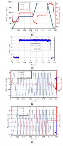
Figure 2. (a) Reference rotor speed, (b) Load torque
Table 2. Parameters of the FIPMSM
|
Parameters |
Units |
Values |
|
Rated voltage (Vdc) |
V |
48 |
|
Rated power |
kW |
8 |
|
Base speed |
rpm |
1300 |
|
Speed-normalized amplitude of 1st harmonic EMF |
V/rad/s |
0.1358 |
|
Speed-normalized amplitude of 3rd harmonic EMF |
V/rad/s |
0.01356 |
|
ψ1, Magnetic flux of the 1st harmonic |
mWb |
19.4 |
|
ψ3, Magnetic flux of the 3rd harmonic |
mWb |
0.675 |
|
Stator resistance |
mΩ |
11 |
|
Lp, Inductance of the main fictitious machine |
µH |
118 |
|
Ls, Inductance of the second fictitious machine |
µH |
51.4 |
|
Pole pairs |
|
7 |
Table 3. Parameters of the SMO for the sensorless control
|
Parameters |
k1 |
k2 |
l1 |
l2 |
a |
|
Values |
250 |
25 |
500 |
1000 |
0.1 |
In this simulation, a special cycle for the reference rotor speed as shown in Figure 2 (a) is considered to verify the stability and robustness of the proposed SMO under the speed and load torque variations. The FIPMSM parameters are provided in Table 2. The SMO parameters are provided in Table 3. The control strategy with id=0 is carried out. In Figure 2 (a), the reference speed is from 0 to 1300 rpm. The application of load torque shown in Figure2 (b) is as follows: 0 Nm at t= [0, 0.03 s], 10 Nm at t= [0.03, 0.19 s] and 0 Nm at t= [0.19, 0.21 s]. It can be noticed that the rotor speed is not required for the torque control, but it is still estimated to verify the feasibility of the proposed SMO.
Figure 3. Simulation waveforms: (a) Actual and estimated fundamental current in α-axis, (c) Actual and estimated current of third harmonic in α-axis, (b) and (d) the error obtained from the estimation of fundamental and third harmonic of current
In Figures 3 and 4, the current and back-EMF observers based on SMO accurately estimate the current and the back-EMF signals of each fictitious machine in wide speed range. Thus, the stability and robustness of the proposed SMO under the torque and speed variations are proved.
Figure 4. Simulation waveforms: (a) Actual and estimated fundamental of back-EMF in α-axis, (c) Actual and estimated third harmonic of back-EMF in α-axis, (b) and (d) The error resulting from the estimation of fundamental and third harmonic of back-EMF
When the amplitude of the back-EMF signal of the main and secondary fictitious machine is low, the estimation process is not precise. Therefore, the estimation of the rotor position in this range will be considered greatly impacted.
In Figure 2 (a), the reference rotor speed cycle contains several transient and steady states, which are used to highlight the effectiveness of the proposed SMO. The estimated currents and back-EMF signals show that the proposed SMO is not impacted when the reference speed changes from steady state to transient state or vice versa.
It is noted that the load torque disturbance also has no obvious effect on the estimation process. The load torque is applied in transient state as in steady state. In fact, it can be seen form the simulation waveforms of Figure 4 that the estimated back-EMF signals of the first and third harmonic components are not affected by the load torque variations.
In Figure 3 (c), the current of the secondary fictitious machine is less than the current in the main fictitious machine. Therefore, the actual and estimated currents of the third harmonic are impacted by the high frequency component of the PWM, especially when the amplitude of the current is low.
Even though the third harmonic of the FIPMSM (parameters provided in Table 2) only accounts for 10% of the first harmonic, the sliding mode observer allows a precise estimation of the back-EMF of the secondary fictitious machine in wide speed range. Thus, it can be concluded that the third harmonic component can be used, in the case of FIPMSM, to estimate the rotor position.
In the following section, actual rotor position, speed and torque will be compared to the estimated ones using the proposed sensorless control based on SMO.
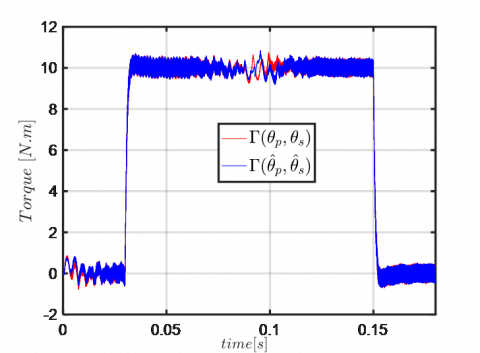
Figure 5 and 6 show the actual and estimated values of the rotor position and speed. The simulations waveforms are obtained for the reference rotor speed and torque given by the Figure 2. In fact, the SMO allows an accurate estimation of the rotor speed in steady state and transient state as shown in Figure 5 (a). From Figure 5 (d), the estimated rotor position $\hat{\theta}_{p}$ through the main fictitious machine converge to the actual one with high accuracy. From Figure 6 (b), the estimated rotor position $\hat{\theta}_{s}$ through the second fictitious machine is also precise. Using the angles $\hat{\theta}_{p}$ and $\hat{\theta}_{s}$ for the sensorless control of the FIPMSM, it can be noticed that the torque converges to the actual one (Figure 5 (b)) obtained when the rotor position is provided by encoder.
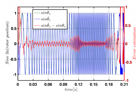
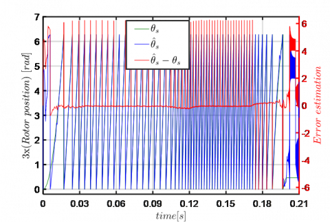
The error between the real and estimated θp, through the main fictitious machine (first harmonic), is less than 1.5 degree as shown in Figure 5 (d). In addition, the error between the real and estimated θs, through the secondary fictitious machine (third harmonic), is less than 6 degrees as shown in Figure 6 (b). This error between the real and estimated position is evaluated in the medium speed range (100-1300 rpm). Therefore, it is concluded that, in the case of FIPMSM, the third harmonic can also be used to perform the sensorless control. However, at zero and low speed range (0-100 rpm), the rotor position estimation is not accurate as in Figures 5 (c)-(d), and Figures 6 (a)-(b). This is due to the low amplitude of the back-EMF at low speed range. In another hand, it should be noted that the pulses present in the position error (Figure 5 (d) and Figure 6 (b)), resulting to the compute of the estimation error, have not any impact on the control loop. This is due to the trigonometric functions used by the Park matrix transformation allowing the compute of currents and voltages components in (d-q) frame.
Figure 5. Simulation waveforms: (a) Actual and estimated rotor speed, (b) the measured torque (using an encoder) and the one (using sensorless) (c) sine actual and estimated rotor position of the main fictitious machine, (d) actual and estimated rotor position of the main fictitious machine
(a)
(b)
(c)
(d)
Figure 6. Simulation waveforms: (a) sine actual and estimated rotor position of the secondary fictitious machine, (b) error between the sine of actual and estimated rotor position of the secondary fictitious machine, (c) Actual and estimated rotor speed during speed reversal, (d) the measured torque (using an encoder) and the one (using sensorless)
From Figure 6 (c) and (d), the robustness of the proposed sensorless control based on SMO during speed reversal is verified. The rotor speed is estimated with accuracy and a good quality of torque under sensorless control mode is achieved.
4.2 Verifying Robustness of the proposed sensorless control
The robustness of the proposed observer, based on SMO, is required to perform an efficient sensorless control of the FIPMSM. In the above section 4.1, the robustness of the observer against speed and torque variation is verified. Thus, the robustness when the parameters of the FIPMSM (resistance, inductance, and flux of permanent magnets) change should be also verified. It is to highlight the efficiency of the proposed sensorless control approach.
The verification of the robustness against the machine parameters variation can be tested by using the defined benchmark given in [24]. The reference rotor speed and the reference torque are shown in Figure 7.
(a)
(b)
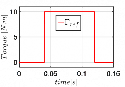
Figure 7. Benchmark used to verify the robustness of the sensorless control: (a) reference rotor speed, (b) reference torque
As defined in the benchmark [24], the resistance as defined in the benchmark [24], the resistance of the machine increases by 50% and decreases by 50%. The inductance increases by 20% and decreases by 20%, and the amplitude of the flux of permanent magnets increases also by 15% and decreases by 15%. This is to introduce a variation in the machine parameters. It is important to be noticed that the parameters variation is only at the machine (FIPMSM), and not on the control system and the SMO. It can be noticed that the machine parameters are affected mostly by the temperature, the saturation and the frequency [25]. The simulation results.
With variations of the resistance and the inductance of the FIPMSM are given respectively in Figures 8 and 9.
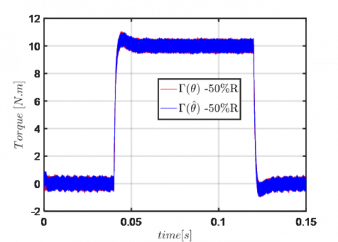
In Figure 8, the resistance variation (due to the variation of the temperature inside the machine) has not an impact on the measured torque. However, the estimated speed when the resistance increases by 50% is not precise especially when the torque increases (Figure 8 (c)). The error estimation value between the actual and estimated rotor speed is 30 rpm when the torque is 10Nm. Thus, it can be concluded that the proposed SMO is robust and can guarantee the sensorless control under an important resistance variation.
(a)
(b)
(c)
Figure 8. Simulation waveforms when the resistance of FIPMSM is changed: (a) the measured torque (using an encoder) and the one (using sensorless) when the resistance decreases by 50%, (b) the measured torque (using an encoder) and the one (using sensorless) when the resistance increases by 50%, (c) Actual and estimated rotor speed when the resistance decreases and increases by 50%
(a)
(b)
(c)
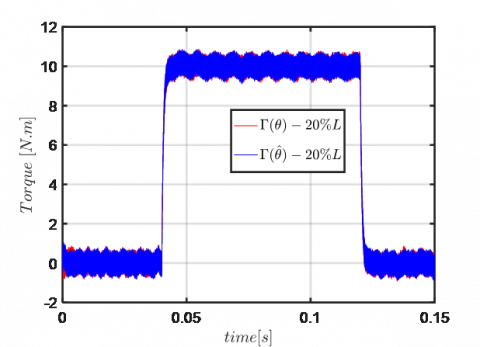
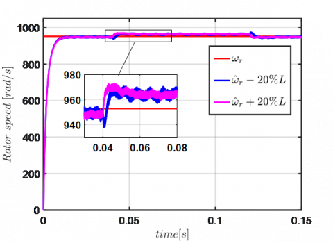
Figure 9. Simulation waveforms when the inductance of FIPMSM is changed: (a) the measured torque (using an encoder) and the one (using sensorless) when the inductance decreases by 20%, (b) the measured torque (using an encoder) and the one (using sensorless) when the inductance increases by 20%, (c) Actual and estimated rotor speed when the inductance decreases and increases by 20%
From Figure 9, the inductance variation (due to the saturation effects of magnetic circuit of the machine) presents no significant impacts on the measured torque. Nevertheless, the error estimation of the rotor speed is not precise when the torque is applied.
The error estimation is less than 20 rpm (Figure 9 (c)), when the inductance increases by 20% and decreases by 20%. So, based on the results in Figure 9, it can be concluded that the proposed SMO is robust and can guarantee the sensorless control under the inductance variation.
(a)
(b)
(c)
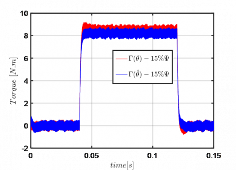
Figure 10. Simulation waveforms when the flux of the permanent magnets of FIPMSM is changed: (a) the measured torque (using an encoder) and the one (using sensorless) when the flux decreases by 15%, (b) the measured torque (using an encoder) and the one (using sensorless) when the flux increases by 15%, (c) Actual and estimated rotor speed when the flux decreases and increases by 15%
Figure 10 shows results under the flux of permanent magnets variation (due to the variation of the magnets temperature). When the amplitude of flux decreases by 15%, the error between the measured torque using an encoder and the one using the proposed sensorless control is less than 6%. And the error when the amplitude of flux increases by 15% is less than 4%. In Figure 10 (c), the estimated rotor speed is greatly affected in both cases, when the flux increases and decreases by 15%. This is due to the estimation process of the rotor speed, that depends directly on the amplitude of the flux as shown in (18). Thus, it can be concluded that the robustness of the proposed SMO is affected under the flux variation of permanent magnets.
In this paper, an observer based on the sliding mode is designed for the sensorless control of a non-sinusoidal back-EMF of FIPMSM. The approach can be easily generalized to a n-phase machine whose electromotive force contains only the harmonics from one to (n-1)/2. On the contrary, the limit of the method is appearing for a five-phase (resp n-phase) machine if harmonic higher than the fifth (resp. the nth) are present. The simulation results show that the proposed SMO estimates the rotor position and speed in a wide speed range with high accuracy. Furthermore, in terms of robustness, the results show that the observer can guarantee the precise sensorless control under the resistance and inductance variation. However, the robustness is impacted under the flux of permanent magnets variation, especially in the rotor speed estimation process. Therefore, the proposed SMO with the consideration of the impact of third harmonic component (in FIPMSM) allows an accurate estimation of the rotor position, as the conventional SMO (with the consideration of only first harmonic). It can be noticed that when the third harmonic is important, the estimation of rotor position through the secondary fictitious machine is more precise. Thus, it can be concluded that the proposed observer can significantly improve the robustness and reliability of the control system by increasing the degrees of freedom for control. Lastly, the proposed SMO sensorless control in this paper does not take into account the low speed range (0-10% of the base speed). Indeed, the developed algorithm is applied to a 48V FIPMSM since 10% of speed leads to a very low back-EMF which cannot be estimated correctly.
This work has been achieved within the framework of CE2I project. CE2I is co-financed by European Union with the financial support of European Regional Development Fund (ERDF), French State and the French Region of Hauts-de-France.
[1] Levi, E. (2008). Multiphase electric machines for variable-speed applications. IEEE Transactions on Industrial Electronics, 55(5): 1893-1909. https://doi.org/10.1109/TIE.2008.918488
[2] Khan, K.S., Arshad, W.M., Kanerva, S. (2008). On performance figures of multiphase machines. In 2008 18th International Conference on Electrical Machines, pp. 1-5. https://doi.org/10.1109/ICELMACH.2008.4799836
[3] Intelligent Integrated Energy Converter project (CE2I). Available: http://ce2i.pole-medee.com/the-project/, accessed on September, 30, 2020.
[4] Burkhardt, Y., Spagnolo, A., Lucas, P., Zavesky, M., Brockerhoff, P. (2014). Design and analysis of a highly integrated 9-phase drivetrain for EV applications. In 2014 International Conference on Electrical Machines (ICEM), pp. 450-456. https://doi.org/10.1109/ICELMACH.2014.6960219
[5] Jahns, T.M., Dai, H. (2017). The past, present, and future of power electronics integration technology in motor drives. CPSS Transactions on Power Electronics and Applications, 2(3): 197-216. https://doi.org/10.24295/CPSSTPEA.2017.00019
[6] Abebe, R., Vakil, G., Calzo, G.L., Cox, T., Lambert, S., Johnson, M., Mecrow, B. (2016). Integrated motor drives: State of the art and future trends. IET Electric Power Applications, 10(8): 757-771.
[7] Hansen, J.F., Wendt, F. (2015). History and state of the art in commercial electric ship propulsion, integrated power systems, and future trends. Proceedings of the IEEE, 103(12): 2229-2242. https://doi.org/10.1109/JPROC.2015.2458990
[8] Vas, P. (1998). Sensorless Vector and Direct Torque Control. Oxford University Press, p. 729.
[9] Benjak, O., Gerling, D. (2010). Review of position estimation methods for IPMSM drives without a position sensor part I: Nonadaptive methods. In The XIX International Conference on Electrical Machines-ICEM, pp. 1-6. https://doi.org/10.1109/ICELMACH.2010.5607978
[10] Zhang, L., Fan, Y., Li, C., Nied, A., Cheng, M. (2017). Fault-tolerant sensorless control of a five-phase FTFSCW-IPM motor based on a wide-speed strong-robustness sliding mode observer. IEEE Transactions on Energy Conversion, 33(1): 87-95. https://doi.org/10.1109/TEC.2017.2727074
[11] Ramezani, M., Ojo, O. (2015). The modeling and position-sensorless estimation technique for a nine-phase interior permanent-magnet machine using high-frequency injections. IEEE Transactions on Industry Applications, 52(2): 1555-1565. https://doi.org/10.1109/TIA.2015.2506143
[12] Parsa, L., Toliyat, H.A. (2007). Sensorless direct torque control of five-phase interior permanent-magnet motor drives. IEEE Transactions on Industry Applications, 43(4): 952-959. https://doi.org/10.1109/TIA.2007.900444
[13] Sun, K., Shi, Y., Huang, L., Li, Y., Xiao, X. (2014). A 2-D fuzzy logic based MRAS scheme for sensorless control of interior permanent magnet synchronous motor drives with cyclic fluctuating loads. In 2014 IEEE Applied Power Electronics Conference and Exposition-APEC, 2014: 2475-2481. https://doi.org/10.1109/APEC.2014.6803651
[14] Michalski, T., Lopez, C., Garcia, A., Romeral, L. (2016). Sensorless control of five phase PMSM based on extended Kalman filter. In IECON 2016-42nd Annual Conference of the IEEE Industrial Electronics Society, pp. 2904-2909. https://doi.org/10.1109/IECON.2016.7793740
[15] Zhang, X., Tian, G., Huang, Y., Lu, Z. (2016). A comparative study of pmsm sensorless control algorithms: Model based vs luenberger observer. In 2016 IEEE Vehicle Power and Propulsion Conference (VPPC), pp. 1-6. https://doi.org/10.1109/VPPC.2016.7791566
[16] Hosseyni, A., Trabelsi, R., Kumar, S., Mimouni, M.F., Iqbal, A. (2017). New sensorless sliding mode control of a five-phase permanent magnet synchronous motor drive based on sliding mode observer. International Journal of Power Electronics and Drive Systems, 8(1): 184-203. https://doi.org/10.1109/VPPC.2016.7791566
[17] Hosseyni, A., Trabelsi, R., Mimouni, M.F., Iqbal, A., Alammari, R. (2015). Sensorless sliding mode observer for a five-phase permanent magnet synchronous motor drive. ISA Transactions, 58: 462-473. https://doi.org/10.1016/j.isatra.2015.05.007
[18] Qiao, Z., Shi, T., Wang, Y., Yan, Y., Xia, C., He, X. (2012). New sliding-mode observer for position sensorless control of permanent-magnet synchronous motor. IEEE Transactions on Industrial Electronics, 60(2): 710-719. https://doi.org/10.1109/TIE.2012.2206359
[19] Yang, J., Dou, M., Zhao, D. (2017). Iterative sliding mode observer for sensorless control of five-phase permanent magnet synchronous motor. Bulletin of the Polish Academy of Sciences. Technical Sciences, 65(6): 845-857. https://doi.org/10.1515/bpasts-2017-0092
[20] Semail, E., Kestelyn, X., & Bouscayrol, A. (2004). Right harmonic spectrum for the back-electromotive force of an n-phase synchronous motor. In Conference Record of the 2004 IEEE Industry Applications Conference, 2004. 39th IAS Annual Meeting, 1: 1-78. https://doi.org/10.1109/IAS.2004.1348390
[21] Semail, E., Bouscayrol, A., Hautier, J.P. (2003). Vectorial formalism for analysis and design of polyphase synchronous machines. The European Physical Journal-Applied Physics, 22(3): 207-220. https://doi.org/10.1051/epjap:2003034
[22] Kim, H., Son, J., Lee, J. (2010). A high-speed sliding-mode observer for the sensorless speed control of a PMSM. IEEE Transactions on Industrial Electronics, 58(9): 4069-4077. https://doi.org/10.1109/TIE.2010.2098357
[23] Chi, W.C., Cheng, M.Y. (2014). Implementation of a sliding-mode-based position sensorless drive for high-speed micro permanent-magnet synchronous motors. ISA Transactions, 53(2): 444-453. https://doi.org/10.1016/j.isatra.2013.09.017
[24] Ghanes, M., Girin, A., Saheb, T. (2004). Original benchmark for sensorless induction motor drives at low frequencies and validation of high gain observer. Proceedings of the 2004 American Control Conference, 1: 71-75. https://doi.org/10.23919/ACC.2004.1383581
[25] Bogado, B., Barrero, F., Arahal, M.R., Toral, S., Levi, E. (2013). Sensitivity to electrical parameter variations of predictive current control in multiphase drives. In IECON 2013-39th Annual Conference of the IEEE Industrial Electronics Society, pp. 5215-5220. https://doi.org/10.1109/IECON.2013.6699982