Attoui Hadjira* | Behih Khalissa | Bouchama Ziyad | Zerroug Nadjat
© 2021 IIETA. This article is published by IIETA and is licensed under the CC BY 4.0 license (http://creativecommons.org/licenses/by/4.0/).
OPEN ACCESS
This paper presents an intelligent monitoring control strategy for a maximum power point tracking (MPPT) in photovoltaic (PV) system applications. The design of the proposed nonlinear adaptive control law (AFBSMC) is formulated based on adaptive fuzzy systems, backstepping approach and sliding mode technique to maximize the power output of a PV system under various sets of conditions and parameters variation. Unlike many conventional controllers, the main contribution of the present paper provides a soften control law which useful to handle parameters variations due to the different operating conditions occurring on the PV system and makes the controller easy to implement. This aim is achieved using fuzzy systems in an adaptive scheme to approximate the switching control function of the global control law while backstepping sliding mode control compensates uncertainties and external disturbances. The analytical stability proof of the closed-loop system is corroborated via Lyapunov synthesis while numerical simulations of different operating conditions of a PV system is conducted to validate the effectiveness of the proposed approach.
backstepping sliding mode control, adaptive fuzzy control, Lyapunov stability, MPPT, photovoltaic system, DC-DC converter
Renewable energy has drawn much attention in recent years due to the high demand for green energy resources. The importance of solar panels (solar energy system) is greater nowadays as renewable sources since they exhibit many merits such as producing clean electrical energy, little maintenance and unlike other sources of renewable energy it has no geographical restrictions.
Solar PV systems have complex configurations that consist of components with nonlinear behaviors mainly due to the weather varying conditions such as temperature, irradiance and among others. These operating conditions are changed significantly with time which requires an adaptive control scheme to maintain adequate maximum power production in a practical operating environment.
Therefore, ensuring maximum electrical power extraction from photovoltaic systems, regardless of load changes and environmental conditions, is the primary objective control strategy, known as the Maximum Power Point Tracking Problem (MPPT) [1].
Many methods have been developed to determine the maximum power point (MPP) under all conditions [2-8]. There are numerous approaches, some of which are based on the well-known perturb and observe (P&O) concept [2, 3], others on the sliding mode control method [4, 5], artificial neural networks or fuzzy based algorithms [6, 7], and synergetic control [1, 7, 8].
Maximum power voltage (MPV)-based techniques using a two-loop MPPT control system are proposed in Refs. [9-11]. The first loop determines the PV array's MPV reference, while the second regulates the PV array's voltage to the reference voltage. The MPV reference search and PV voltage tracking are repeated until the maximum power is obtained. A hybrid technique consisting of two loops is presented in Ref. [12] to track MPP more effectively. MPP is estimated using an incremental conductance approach in the first loop. To regulate the system to the searched reference MPP, a second loop terminal sliding mode controller is constructed. Whereas Dahech et al. [13] proposed backstepping sliding mode control (BSMC) for the second loop. However, the main drawback of the SMC is the chattering. We propose in this paper to approximate discontinuous control using an adaptive fuzzy system based on the universal approximation theorem to tackle the problem of chattering mentioned in Ref. [13]. To ensure the system's global stability, the parameter of the fuzzy system is modified using an adaptation law based on the Lyapunov synthesis.
The goal of this work is to develop an adaptive fuzzy Backstepping sliding mode controller (AFBSMC) for MPPT, in order to overcome the problem of chattering. The whole system is modeled and simulated in Matlab/Simulink. Simulation results prove and confirm the effectiveness of the proposed approach in the elimination of the chattering.
The performance of this approach proves a high efficiency compared to the BSMC. The remainder of this paper is organized as follows. In Section 2, the MPPT system modeling is presented. The design of AFBSMC is exposed in Section 3. Section 4 uses numerical simulations to demonstrate the controller's usefulness in tracking MPP. The paper comes to a close with a conclusion.
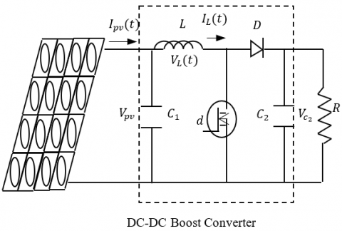
Consider a boost type converter connected to a PV module with a resistive load as illustrated in Figure 1.
Figure 1. MPPT system schematic
2.1 PV model
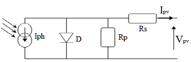
PV array is a p-n junction semiconductor, which converts light into electricity. When the incoming solar energy exceeds the band-gap energy of the module, photons are absorbed by materials to generate electricity. The equivalent-circuit model of PV is shown in Figure 2.
It consists of a light-generated source, diode (D), series and parallel resistances [14].
Figure 2. Equivalent model of solar cell
where Iph indicates photocurrent, which depends on the level of light intensity, Ipv (Photovoltaic panel current) is output current, Vpv is the PV module output voltage, Rp is the equivalent shunt resistance, and Rs is the intrinsic series resistance.
In this work the PV module used is the KC200GH-2P. The parameters of this module are exposed in Table 1.
Figures 3 and 4 show the PV characteristic under different irradiance levels, and under different temperatures respectively.
As illustrated in the figures, the open-circuit voltage is dominated by temperature, and solar irradiance has preeminent influence on short- circuit current (Isc). We can conclude that high temperature and low solar irradiance will reduce the power conversion capability.
Table 1. Parameters of the PV module KC200GH-2P
|
Parameter |
Value |
|
Maximum power Pmpp |
200 [W] |
|
Short circuit current Iscr |
8.21 [A] |
|
Open circuit voltage Voc |
32.9 [V] |
|
Voltage at maximum power point Vmpp |
26.3 [V] |
|
Current at maximum power point Impp |
7.61 [A] |
|
P-N junction characteristic factor A |
1.8 |
Figure 3. PV characteristic under different irradiances levels (temperature =25°C)
Figure 4. PV characteristic under diffe
2.2 Boost converter model
The converter is used to regulate the PV module output voltage Vpv in order to extract as much power as possible from the PV module. Referring to Ref. [12], the dynamics of the boost converter is given by Eq. (1):
$\frac{d V_{p v}}{d t}=\frac{1}{C_{1}}\left(I_{p v}-I_{L}\right)$
$\frac{d I_{L}}{d t}=\frac{1}{L} V_{p v}-\frac{R_{C}(1-d)}{L\left(1+\frac{R_{C}}{R}\right)} I_{L}$
$+\frac{1-d}{L}\left(\frac{R_{C}}{R_{C}+R}-1\right) V_{C 2}-\frac{V_{D}(1-d)}{L}$
$\frac{d V_{C 2}}{d t}=\frac{1-d}{C_{2}\left(1+\frac{R_{C}}{R}\right)} I_{L}-\frac{1}{C_{2}\left(R_{C}+R\right)} V_{C 2}$ (1)
where, the three state variables Vpv, IL and VC2 are respectively the output voltage of the PV module, the inductor current and the voltage of the capacitor C2. VD is the forward voltage of the power diode; d is the duty ratio of the PWM control input signal; R is the load resistance.
By taking $x(t)=\left[V_{p v}(t) I_{L}(t) V_{C 2}(t)\right]^{T}$, the Eq. (1) can be written in the following form [12].
$\left\{\begin{array}{c}\frac{d V_{p v}}{d t}=\frac{1}{C_{1}}\left(I_{p v}-I_{L}\right) \\ \frac{d I_{L}}{d t}=f_{1}(x)+g_{1}(x) d(t) \\ \frac{d V_{C 2}}{d t}=f_{2}(x)+g_{2}(x) d(t)\end{array}\right.$ (2)
where, $x=\left[\begin{array}{lll}x_{1} & x_{2} & x_{3}\end{array}\right]^{T}$.
Eqns. (3)-(6) show the expression of the functions $f_{1}, f_{2}, g_{1}$ and $g_{2}$
$f_{1}(x)=\frac{x_{1}}{L}-\frac{R_{C}}{L\left(1+\frac{R_{C}}{R}\right)} x_{2}+\frac{1}{L}\left(\frac{R_{C}}{R_{C}+R}-1\right) x_{3}-\frac{V_{D}}{L}$ (3)
$g_{1}(x)=-\frac{R_{C}}{L\left(1+\frac{R_{C}}{R}\right)} x_{2}-\frac{1}{L}\left(\frac{R_{C}}{R_{C}+R}-1\right) x_{3}+\frac{V_{D}}{L}$ (4)
$f_{2}(x)=\frac{1}{C_{2}\left(1+\frac{R_{C}}{R}\right)} x_{2}-\frac{1}{C_{2}\left(R_{C}+R\right)} x_{3}$ (5)
$g_{2}(x)=-\frac{1}{C_{2}\left(1+\frac{R_{C}}{R}\right)} x_{2}$ (6)
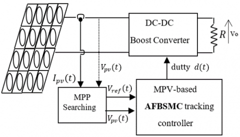
To achieve MPP under the changing atmosphere, the Figure 5 illustrates the overall control structure. Here, Ipv and Vpv are measured from PV array and sent to the MPP searching algorithm, which generates the reference maximum power voltage $V_{\text {ref }}$. Then, the reference voltage $V_{\text {ref }}$ is given to the maximum power voltage based AFBSM controller for the maximum power tracking.
Figure 5. Proposed system
3.1 MPP searching algorithm
To achieve the maximum power operation, we use an incremental conductance method to search the MPP voltage $V_{\text {ref }}$.
The power slope $d P_{p v} / d V_{p v}$ can be expressed as:
$\frac{d P_{p v}}{d V_{p v}}=I_{p v}+V_{p v} \frac{d I_{p v}}{d V_{p v}}$
When the power slope $\frac{d P_{p v}}{d V_{p v}}=0$, i.e., $\frac{d i_{p v}}{d V_{p v}}=-\frac{I_{p v}}{V_{p v}}$, the PV system operates at the maximum power generation.
Therefore, the update law for $V_{\text {ref }}$ is given by the following rules [12]:
$\left\{\begin{array}{l}V_{r e f}=V_{r e f}(k-1)+\Delta V, \text { for } \frac{d i_{p v}}{d V_{p v}}>-\frac{I_{p v}}{V_{p v}} \\ V_{r e f}=V_{r e f}(k-1)-\Delta V, \text { for } \frac{d i_{p v}}{d V_{p v}}<-\frac{I_{p v}}{V_{p v}}\end{array}\right.$
3.2 Backstepping sliding mode controller
To extract the maximum power from a PV panel a backstepping sliding mode controller is designed. Where the objective of this is to let the panel PV voltage $V_{p v}$ track the reference maximum power voltage $V_{\text {ref }}$ by acting on the duty cycle $d(t)$ of the boost converter switch.
The recursive nature of the propose control design is similar to the standard Backstepping methodology. However, the proposed control design uses Backstepping to design controllers with a zero-order sliding surface at the last step [13]. The design proceeds as follows:
For the first step we consider zero-order sliding surface represented by following equation:
$e_{1}=x_{1}-x_{d}$ (7)
where: $x_{d}=V_{\text {ref }}$.
Considering an auxiliary tracking error variable:
$e_{2}=\dot{e}_{1}+\alpha_{1}$ (8)
Let the first Lyapunov function candidate:
$V_{1}=\left(\frac{1}{2}\right) e_{1}^{2}$ (9)
The time derivation of Eq. (5) is given by the Eq. (10):
$\dot{V}_{1}=e_{1} \dot{e}_{1}=e_{1}\left(e_{2}-\alpha_{1}\right)=-\lambda_{1} e_{1}^{2}+e_{1} e_{2}$ (10)
The stabilization of $\mathrm{e}_{1}$ can be obtained by introducing a new virtual control $\alpha_{1}$ Eq. (11), such that:
$\alpha_{1}=\lambda_{1} e_{1}, \lambda_{1}>0$ (11)
where $\lambda_{1}$ a positive feedback gain, such that $\alpha_{1}$ has been chosen in order to eliminate the non linearity and getting $\dot{V}_{1}(s)<0$. The term $e_{1} e_{2}$ of $\dot{V}_{1}$ will be eliminated in the next step, so the first sub system is stabilized.
For the second step we consider the following sliding surface:
$s=\lambda_{2} e_{1}-e_{2}$ (12)
The augmented Lyapunov function is given by Eq. (13):
$V_{2}=V_{1}+\left(\frac{1}{2}\right) s^{2}$ (13)
Eqns. (14)-(15) show the time derivative of $V_{2}$:
$\dot{V}_{2}=\dot{V}_{1}+s . \dot{s}$ (14)
$\dot{V}_{2}=-\lambda_{1} e_{1}^{2}+e_{1} e_{2}+s .\left[\lambda_{2}\left(e_{2}-\lambda_{1} e_{1}\right)-\dot{e}_{2}\right]$ (15)
The Eqns. (16)-(18) represent the time derivative of $e_{2}$:
$\dot{e}_{2}=\ddot{e}_{1}+\dot{\alpha}_{1}$ (16)
$\dot{e}_{2}=\ddot{V}_{p v}-\ddot{x}_{1 d}+\dot{\alpha}_{1}$ (17)
$\dot{e}_{2}=-\frac{1}{C_{1}}\left[f_{1}(x)+g_{1}(x) d(t)\right]+\frac{1}{C_{1}} \dot{I}_{p v}-\ddot{x}_{1 d}+\dot{\alpha}_{1}$ (18)
One can obtain the Eq. (19):
$\dot{s}=\left[\lambda_{2}\left(e_{2}-\lambda_{1} e_{1}\right)+\frac{1}{C_{1}}\left[f_{1}(x)+g_{1}(x) d(t)\right]\right.$
$\left.-\frac{1}{C_{1}} I_{p v}+\ddot{x}_{1 d}-\dot{\alpha}_{1}\right]$ (19)
We impose the following dynamic to the sliding surface:
$\dot{s}=-h \cdot(s+\beta \operatorname{sgn}(s))$ (20)
$\operatorname{sign}(.)$ is the usual sign function., where $h>0$ and $\beta>0$ .
Substituting Eq. (18) into Eq. (15) we obtain:
$\begin{aligned} \dot{V}_{2}=-\lambda_{1} \mathrm{e}_{1}^{2}+\mathrm{e}_{1} \mathrm{e}_{2} & \\+& \mathrm{s}\left[\lambda_{2}\left(e_{2}-\lambda_{1} e_{1}\right)\right.\\ &-\left(-\frac{1}{C_{1}}\left[f_{1}(x)+g_{1}(x) d(t)\right]\right.\\ &\left.\left.+\frac{1}{C_{1}} I_{p v}-\ddot{x}_{1 d}+\dot{\alpha}_{1}\right)\right] \end{aligned}$ (21)
The control law is defined as:
$d(t)=d_{e q}(t)+\frac{C_{1}}{g_{1}(x)} d_{s w}(t)$ (22)
$d_{s w}(t)=-h(s+\beta \operatorname{sgn}(s))$ (23)
where, $d_{s w}(t)$ in the Eq. (23) is the switching control.
So we have:
$d(t)=\frac{1}{g_{1}(x)}\left[-f_{1}(x)-C_{1} \lambda_{2}\left(e_{2}-\lambda_{1} e_{1}\right)+I_{p v}\right.$$-C_{1} \ddot{x}_{1 d}+C_{1} \dot{\alpha}_{1}-C_{1} h(\mathrm{~s}$$+\beta s g n(s)]$ (24)
The Eq. (15) is developed to:
$\dot{V}_{2}=-\lambda_{1} e_{1}^{2}+e_{1} e_{2}-s[h(\mathrm{~s}+\beta \operatorname{sgn}(s)]$ (25)
Introducing the norm in the Eq. (25), we get the Eqns. (26) and (27):
$\dot{V}_{2} \leq-\lambda_{1} e_{1}^{2}+e_{1} e_{2}-h s^{2}-\beta|s|$ (26)
$\dot{V}_{2} \leq-e^{T} p e-\beta|s|$ (27)
where, $e=\left[\begin{array}{ll}e_{1} & e_{2}\end{array}\right]^{T}$and P is a symmetric matrix defined as:
$P=\left[\begin{array}{cc}\lambda_{1}+h \lambda_{2}^{2} & -h \lambda_{2}-\frac{1}{2} \\ -h \lambda_{2}-\frac{1}{2} & h\end{array}\right]$
This proves the decreasing of Lyapunov function, which ensures that the closed-loop system is stable and robust.
This kind of sliding mode is certainly robust and stabilized but has two major drawbacks. The first lies in the presence of the sign function, where the control signal causes the phenomenon of chattering. The second disadvantage lies in the difficulty of the calculation of the constant $\beta, h$. To overcome these drawbacks several solutions have been presented in literature [15-17].
In order to resolve this problem, we propose to modify the following in the previous control law by using a fuzzy adaptive system. By letting the sliding area has input to approximate the term $d_{s w}(t)$. The fuzzy kind of lathing allows elimination of the phenomenon of chattering perfectly. At the same time as the adaptive appearance is designed to approximate the constant.
3.3 AFBSM controller of PV system
In this work we use the following If-Then rules [18, 19] to construct the fuzzy logic system:
$R_{i}:$ If $x_{1}$ is $F_{1}^{i}$ and ... and $x_{n}$ is $F_{n}^{i}$ then $y$ is $B^{i}, i=1,2, \ldots, n$
The fuzzy logic system with the singleton fuzzifier, product inference and center average defuzzifier is written as follows:
$y(x)=\frac{\sum_{i=1}^{n} \theta_{i} \prod_{j=1}^{n} \mu_{F_{j}^{i}\left(x_{j}\right)}}{\sum_{i=1}^{n}\left[\prod_{j=1}^{n} \mu_{F_{j}^{i}}\left(x_{j}\right)\right]}$ (28)
where,
$x=\left[x_{1}, \ldots, x_{n}\right]^{T} \in R^{n}, \mu_{F_{j}^{i}}\left(x_{j}\right)$ is the membership of $F_{j}^{i}$
$\theta_{i}=\max _{y \in R} \mu_{B^{i}}(y)$, let:
$\xi_{i}(x)=\frac{\prod_{j=1}^{n} \mu_{F_{j}^{i}}\left(x_{j}\right)}{\sum_{i=1}^{n}\left[\prod_{j=1}^{n} \mu_{F_{j}^{i}}\left(x_{j}\right)\right]}$ (29)
$\xi(x)=\left[\xi_{1}(x), \xi_{2}(x), \ldots, \xi_{n}(x)\right]^{T}$ and $\theta=\left[\theta_{1}, \theta_{2}, \ldots, \theta_{n}\right]^{T}$.
Then the fuzzy logic system can be rewritten by the Eq. (30):
$y(x)=\theta^{T} \xi(x)$ (30)
The following Lemma, points out that the above fuzzy logic systems are capable to uniformly approximating any continuous nonlinear function, over a compact set Ωx.
Lemma: [18-19].
For any given continuous function f(x) on a compact set $\Omega_{x} \subset R^{n}$; there exists a fuzzy logic system y(x) In the form (30), such that for any given positive constant ε.$\sup _{x \in \Omega_{x}}|f(x)-y(x)| \leq \varepsilon$.
Then we propose to use a fuzzy system in the form (30) which can approximate the discontinuous control $d_{s w}(x)$, this latter is modeled by fuzzy system $\hat{h}(s)$. Then we have the following Eqns. (31) and (32):
$d_{s w}(x)=\hat{z}(s)+\Delta z(x)$ (31)
$\hat{z}(s)=\hat{\theta}_{z}^{T} \xi_{z}(s)$ (32)
Such that: w= Δz(x), is the approximation error.
So the control law is:
$d(t)=\frac{1}{g_{1}(x)}\left[-f_{1}(x)-C_{1} \lambda_{2}\left(e_{2}-\lambda_{1} e_{1}\right)+\dot{I}_{p v}\right.$
$\left.-C_{1} \ddot{x}_{1 d}+C_{1} \dot{\alpha}_{1}-C_{1} \hat{z}(s)\right]$ (33)
The augmented Lyapunov function is given by Eq. (34):
$V_{2}=V_{1}+\left(\frac{1}{2}\right) s^{2}+\frac{1}{2 \eta_{z}} \tilde{\theta}_{z}^{T} \tilde{\theta}_{z}$ (34)
The derivative of this latter introducing Eq. (31), is given by Eqns. (35) and (36):
$\dot{V}_{2}=-\lambda_{1} e_{1}^{2}+e_{1} e_{2}+s \cdot\left[\lambda_{2}\left(e_{2}-\lambda_{1} e_{1}\right)-(-\frac{1}{C 1}\left[f_{1}(x)+g_{1}(x)\left(d_{e q}(t)\right)\right]+\tilde{\theta}_{z} \xi(s) \underbrace{-\hat{z}(s)}+w+\frac{1}{C 1} \dot{I}_{p v}-\ddot{x}_{1 d}+\dot{\alpha}_{1})\right]-\frac{1}{\eta_{h}} \tilde{\theta}_{z}^{\tau} \hat{\theta}_{z}$ (35)
$\dot{V}_{2}=-\lambda_{1} e_{1}^{2}+e_{1} e_{2}+s \cdot\left[\lambda_{2}\left(e_{2}-\lambda_{1} e_{1}\right)-(-\frac{1}{\mathrm{C} 1}\left[f_{1}(x)+g_{1}(x)\left(d_{e q}(t)\right)\right] \underbrace{-\hat{z}(s)}+w+\frac{1}{C 1} \dot{I}_{p v}-\ddot{x}_{1 d}+\dot{\alpha}_{1})\right]-\frac{1}{\eta_{h}} \tilde{\theta}_{z}^{T}\left[\dot{\hat{\theta}}_{z}-\eta_{z} s \cdot \xi(s)\right]$ (36)
Choosing the adaptive law as follow:
$\dot{\hat{\theta}}_{z}=\eta_{z} s \xi(s)$ (37)
The optimal value of $\hat{z}(s)$ is such that:
$\left|\hat{z}^{*}(s)\right| \geq|w|$ (38)
The Eq. (34) is developed to:
$\dot{V}_{2} \leq=-\lambda_{1} e_{1}^{2}+e_{1} e_{2}+|s|\left[-\left|\hat{z}^{*}(s)\right|+|w|\right]$ (39)
$\dot{V}_{2} \leq-e^{T} Q e-\varphi|s| \rightarrow \dot{V}_{2} \leq 0$ (40)
where,
$\varphi=\left|\hat{z}^{*}(s)\right|-|w|$.
$e=\left[\begin{array}{ll}e_{1} & e_{2}\end{array}\right]^{T}$ and Q is a symmetric matrix with the following form:
$Q=\left[\begin{array}{cc}\lambda_{1}^{2} & -\frac{1}{2} \\ -\frac{1}{2} & 0\end{array}\right]$
This proves the decreasing of Lyapunov function, which ensures that the closed-loop system is stable and robust.
To validate the proposed approach, we used the PV module KC200GH-2P, a boost converter and a resistive load.
We consider that the parameters of the boost are as follows:
L = 1.21 mH, RL = 0.15 Ω, RC = 39.6 Ω, C1 = 1000 µF, C2 = 1000 µF, R = 25 Ω, and VD = 0.82 V.
In this section we present the simulation results when applying the BSMC MPPT controller [16] and the Adaptive Fuzzy Backstepping Sliding Mode control law under different atmospheric conditions and load variation using Matlab/Simulink.
In order to construct the fuzzy system for the signal, we divide the discourse universe (the surface) in to three sets; “Positive”, “Zero” and “Negative” which are associated with the following membership functions Eqns. (41)-(43):
$\mu_{\text {negative }}(s)=1 /(1+8 \cdot \exp (s-0.1))$ (41)
$\mu_{\text {zero }}(s)=1 /\left(-\exp (s / 0.5)^{2}\right)$ (42)
$\mu_{\text {positive }}(s)=1 /(1-8 . \exp (s-0.1))$ (43)
To deduce the signal h ̂(S) we used the Three fuzzy rules:
$\begin{array}{ccccc}R^{1}: \text { if } & \boldsymbol{s} & \text { is } & \text { Negative } & \text { then } & \hat{\mathrm{z}}(s)=-C \\ R^{2}: \text { if } & s & \text { is } & \text { Zero } & \text { then } & \hat{z}(s)=0 \\ R^{3}: \text { if } & s & \text { is } & \text { Positive } & \text { then } & \hat{z}(s)=C\end{array}$
4.1 Simulation results with standard operating conditions
Simulation results at Standard Test Condition: S=1000 W/m² and T = 25°C for both types of control, BSMC MPPT and the proposed AFBSMC are illustrate in Figures 6-9.
Figure 6. Evolution of $P_{P v}$
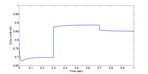
Figure 7. Evolution of duty cycle $d(t)$
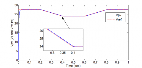
Figure 8. Evolution of $V_{P v}$ and $V_{r e f}$
Figure 9. Evolution of sliding surface
For all the simulation results above, the fuzzy adaptive backstepping sliding mode control approach is able to maintain the output at optimum point and provides a good performance but also rejects the chattering drawback appeared in backstepping sliding mode control.
4.2 Simulation results under irradiation variations
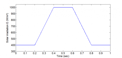
For verifying the effect of changing irradiation conditions, as shown in Figure 10. The temperature is considered constant with a value of 25°C.
As shown in Figures 11-13 below, when the irradiance level changes, the proposed controller can track quickly the maximum power point (the response time of the AFBSMC is 0.02s).
Figure 10. Irradiation's variation
Figure 11. Evolution of $V_{P v}$ and $V_{r e f}$
Figure 12. Evolution of $P_{P v}$
Figure 13. Evolution of duty cycle d(t)
Figure 14. $V_{P v}-P_{P v}$ characteristics under solar irradiation variations
During the simulation the trace of the operating point is staying close to the MPP as shown in Figure 14.
4.3 Simulation results under temperature variations
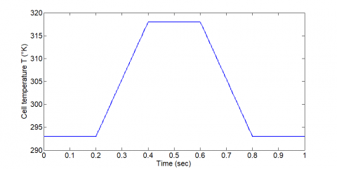
For verifying the effect of changing temperature conditions, as shown Figure 15. The solar irradiation is considered constant with a value of 1000 W/m².
It is clear from Figures 16-18 below that the proposed AFBSMC provides a good performance and proves a high efficiency compared to the BSMC.
Figure 19 illustrates that the proposed controller follows the trajectory of the MPP perfectly.
Figure 15. Temperature’s variation
Figure 16. Evolution of $V_{P v}$ and $V_{r e f}$
Figure 17. Evolution of $P_{P v}$
Figure 18. Evolution of duty cycle d(t)
Figure 19. $V_{P v}-P_{P v}$ characteristics under temperature variations
4.4 Simulation results under load variations
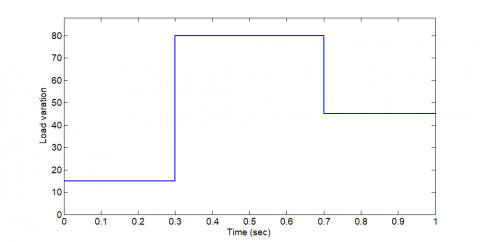
To show the robustness of the proposed AFBSMC, considering load change from 15 Ω to 80 Ω and from 80 Ω to 45 Ω under the Standard Test Condition (S=1000 W/m² and T = 25°C), the corresponding results are shown in Figures 20-22. It can be easily concluded that the proposed controller achieves strong robustness and has satisfactory response under these types of disturbance.
We constate that the AFBSMC not only performs its principal motion to drive the dynamics of the system to operate in the desired performance but also rejects the chattering drawback appeared in BSMC.
Figure 20. Load variation
Figure 21. $P_{P v}$ and $V_{o}$ under load variation
Figure 22. Evolution of duty cycle $d(t)$
This paper develops an adaptive MPPT control algorithm to extract and maximize the power created from PV system. Hence, the design of the proposed controller is based on fuzzy logic systems to generate a continuous time varying duty cycle for a DC converter which is inserted between the PV system and the load. Backstepping sliding mode methodology was derived based on the Lyapunov theory to render the controller more robust and to provide global system stability. The effectiveness and the robustness of the proposed approach have been verified using Simulink software. The obtained results show that the proposed control scheme is indeed appropriate for experimental applications.
[1] Attoui, H., Khaber, F., Melhaoui, M., Kassmi, K., Essounbouli, N. (2016). Development and experimentation of a new MPPT synergetic control for photovoltaic systems. Journal of Optoelectronics and Advanced Materials, 18(1-2): 165-173.
[2] Gradella, V.M., Rafael, G.J., Ruppert, F.E. (2009). Analysis and simulation of the P&O MPPT algorithm using a linearized PV array model. 2009 35th Annual Conference of IEEE Industrial Electronics, pp. 231-236. https://doi.org/10.1109/IECON.2009.5414780
[3] Elgendy, M.A., Zahawi, B., Atkinson, D.J. (2012). Evaluation of perturb and observe MPPT algorithm implementation techniques. In 6th IET International Conference on Power Electronics, Machines and Drives (PEMD 2012), pp. 1-6. https://doi.org/10.1049/cp.2012.0156
[4] El Idrissi, R., Abbou, A., Mokhlis, M. (2020). Backstepping integral sliding mode control method for maximum power point tracking for optimization of PV system operation based on high-gain observer. International Journal of Intelligent Engineering and Systems, 13(5): 133-144. https://doi.org/10.22266/ijies2020.1031.13
[5] Mohammadinodoushan, M., Abbassi, R., Jerbi, H., Ahmed, F. W., Rezvani, A. (2021). A new MPPT design using variable step size perturb and observe method for PV system under partially shaded conditions by modified shuffled frog leaping algorithm-SMC controller. Sustainable Energy Technologies and Assessments, 45: 101056. https://doi.org/10.1016/j.seta.2021.101056
[6] Loukil, K., Abbes, H., Abid, H., Abid, M., Toumi, A. (2020). Design and implementation of reconfigurable MPPT fuzzy controller for photovoltaic systems. Ain Shams Engineering Journal, 11(2): 319-328. https://doi.org/10.1016/j.asej.2019.10.002
[7] Akoro, E., Tevi, G.J., Faye, M.E., Doumbia, M.L., Maiga, A.S. (2020). Artificial neural network photovoltaic generator maximum power point tracking method using synergetic control algorithm. International Journal on Emerging Technologies, 11(2): 590-594.
[8] Nguimfack-Ndongmo, J., Kenné, G., Kuate-Fochie, R., Njomo, A.F.T., Nfah, E.M. (2021). Adaptive neuro-synergetic control technique for SEPIC converter in PV systems. International Journal of Dynamics and Control, 1-14. https://doi.org/10.1007/s40435-021-00808-1
[9] Kim, I.S. (2007). Robust maximum power point tracker using sliding mode controller for the three-phase grid-connected photovoltaic system. Solar energy, 81(3): 405-414. https://doi.org/10.1016/j.solener.2006.04.005
[10] Koutroulis, E., Kalaitzakis, K., Voulgaris, N.C. (2001). Development of a microcontroller-based, photovoltaic maximum power point tracking control system. IEEE Transactions on Power Electronics, 16(1): 46-54. https://doi.org/10.1109/63.903988
[11] Veerachary, M., Senjyu, T., Uezato, K. (2003). Neural-network-based maximum-power-point tracking of coupled-inductor interleaved-boost-converter-supplied PV system using fuzzy controller. IEEE Transactions on Industrial Electronics, 50(4): 749-758. https://doi.org/10.1109/TIE.2003.81476
[12] Chiu, C.S., Ouyang, Y.L., Ku, C.Y. (2012). Terminal sliding mode control for maximum power point tracking of photovoltaic power generation systems. Solar Energy, 86(10): 2986-2995. https://doi.org/10.1016/j.solener.2012.07.008
[13] Dahech, K., Allouche, M., Damak, T., Tadeo, F. (2017). Backstepping sliding mode control for maximum power point tracking of a photovoltaic system. Electric Power Systems Research, 143: 182-188. https://doi.org/10.1016/j.epsr.2016.10.043
[14] Rekioua, D., Matagne, E. (2012). Optimization of Photovoltaic Power Systems: Modelization, Simulation and Control. Springer Science & Business Media.
[15] Lin, W.S., Chen, C.S. (2002). Robust adaptive sliding mode control using fuzzy modelling for a class of uncertain MIMO nonlinear systems. IEE Proceedings-Control Theory and Applications, 149(3): 193-201. https://doi.org/10.1049/ip-cta:20020236
[16] Hamzaoui, A., Essounbouli, N., Zaytoon, J. (2003). Fuzzy sliding mode control for uncertain SISO systems. In IFAC Conf. on Intelligent Control Systems and Signal Processing (ICONS’03), pp. 231-236.
[17] Al-Khazraji, A., Essounbouli, N., Hamzaoui, A., Nollet, F., Zaytoon, J. (2011). Type-2 fuzzy sliding mode control without reaching phase for nonlinear system. Engineering Applications of Artificial Intelligence, 24(1): 23-38. https://doi.org/10.1016/j.engappai.2010.09.009
[18] Wang, L.X. (1992). Fuzzy systems are universal approximators. In 1992 Proceedings IEEE International Conference on Fuzzy Systems, pp. 1163-1170. https://doi.org/10.1109/FUZZY.1992.258721
[19] Castro, J.L. (1995). Fuzzy logic controllers are universal approximators. IEEE Transactions on Systems, Man, and Cybernetics, 25(4): 629-635. https://doi.org/10.1109/21.370193