Mecifi Mohammed* | Boumediene Abdelmadjid | Boubekeur Djamila
© 2021 IIETA. This article is published by IIETA and is licensed under the CC BY 4.0 license (http://creativecommons.org/licenses/by/4.0/).
OPEN ACCESS
The aim of this paper is the control of electric powered wheelchairs (EPW) which was made for people suffering of temporary or permanent disabilities due to illnesses or accidents. The EPW is powered by two Permanent Magnet Synchronous Motors (PMSM) that are characterized by high efficiency, high torque, low noise and robustness; hence the dynamic model of the both EPW-motors is presented in the first. After that, a comparative study is made between two nonlinear command theory; Integrator Backstepping based on the second method of Lyapunov which combine the choice of the energy function with the laws control, and, fuzzy logic introduced to approach human reasoning with the help of an adequate representation of knowledge. To evaluate the performance of the two controls, numerical simulations are presented to show the evolution of electrical and mechanical quantities, the energy consumed and the squared error of the displacement and velocity. However, the reference trajectory used is that generated by the fifth-degree polynomial interpolation, which ensures a regular trajectory that is continuous in positions, velocities and accelerations.
electric powered wheelchair, PMSM, modelling, fuzzy logic, control, trajectory generation, integrator backstepping, tracking trajectory
People who suffer from lower and upper extremity impairments face serious complications to autonomously move in their daily lives. However, a large number of research projects which propose different powered wheelchair control systems are arising.
The electric wheelchair is a unicycle robot with two driving wheels and two idle ones, kinematic and dynamic modelling confirms its multivariate nonlinear nature [1]. It is an electromechanical system whose complete analysis calls together the main disciplines: mechanics, electromechanics, power electronics, automatic, computer science [2].
However, electric motor and navigational controls are the essential parts for the electric powered wheelchair moving. Several strategies have focused on the EPW’s velocity and direction control using different kinds of motors such as DC Motor [3], PMSM [4], brushless DC motors. We can find several examples in previous works such as adaptive controller [5], neural control techniques [6], robust controllers [7, 8], sliding mode [9, 10], backstepping [3], and fuzzy logic [11-14].
The main purpose of this paper is to apply integrator backstepping nonlinear controller based on the second method of Lyapunov which combine the choice of the energy function with the laws control, in the first case. After that, the application of the fuzzy logic nonlinear controller with a generated trajectory reference.
The interest of fuzzy logic lies in its ability to deal with the imprecise, the uncertain and the blurred. It stems from man's ability to decide and act appropriately despite the lack of available knowledge. Indeed, fuzzy logic has been introduced to approach human reasoning with the help of an adequate representation of knowledge [15-19]. The main advantages of fuzzy logic controllers are: simplicity and flexibility; can handle problems with imprecise and incomplete data; can model nonlinear functions of arbitrary complexity; cheaper to develop and can cover a wider range of operating conditions, more readily customizable in natural language terms. Thereafter, a comparative study of the two controllers is done.
After introduction section, the organization of the paper is as follows: section 2 covers the dynamic modelling of EPW based on PMSM actuator. After that, integrator backstepping and fuzzy logic control applied to the global system is proposed in section 3 and 4. Simulations and result analysis are carried out in section 5. Finally, we draw conclusions in section 6.
The dynamic model of the electric wheelchair is essential for the controller design and simulation analysis, it is determined based on the Lagrange method, taking into consideration the different forces that affect its motion unlike kinematics model where the forces are not taken into consideration.
Lagrange dynamics approach is a very powerful method for formulating the motion equations of mechanical systems. This method, which was introduced by Lagrange, is used to systematically derive the equations of motion by considering the kinetic and potential energies of the given system [10, 20].
To analyze the motion of this system; a fixed coordinate O-xy has been assigned as shown in Figure 1.
Figure 1. Wheelchair model going up a slope
Terms used in this part have the meaning summarized in Table 1.
Table 1. Parameters of the EPW
|
Symbol |
Description |
Value |
|
V |
Longitudinal velocity of the EPW |
m/s |
|
ar, al |
Rotational angle of the right/left wheel |
rad |
|
$\alpha_{m r}, \alpha_{m l}$ |
Rotational angle of the right/left motor |
rad |
|
$C_{e m r}, C_{e m l}$ |
Electromagnetic torques of the right/left motor |
N·m |
|
$C_{F r}, C_{F l}$ |
Torque applied on the right/left wheel |
N·m |
|
Cr, Cl |
Load torques required of the right/left motor |
N·m |
|
$\Omega_{r}, \Omega_{l}$ |
Angular rotor velocities of the right/left motor |
Rad/s |
|
Id, Iq |
d- and q-axis stator currents |
A |
|
Vd, Vq |
d- and q-axis stator voltages |
V |
|
M |
EPW with operator mass |
210 kg |
|
Mw |
Mass of driving wheel |
2 kg |
|
L |
Distance between the two driving wheels |
0.57 m |
|
l |
Length of the EPW |
0.87 m |
|
R |
Radius of the driving wheel |
0.17 m |
|
J |
Moment of inertia of the EPW |
16.08 kg.m2 |
|
Jw |
Moment of inertia of the driving wheel |
0.0289 kg.m2 |
|
g |
Acceleration due to gravity |
9.81 m/s2 |
|
$\psi$ |
Slope angle |
% |
|
fw |
Viscous friction coefficient of the wheel |
0.008 N.m.s/rad |
|
$\sigma$ |
Gear ratio |
0.03 |
|
Ja |
Moment of inertia of the motor |
0.0008 kg.m2 |
|
fv |
Viscous friction coefficient of the motor |
0.00005 N.m.s/rad |
|
Rs |
Per phase stator resistance |
2.56 Ω |
|
Ld |
d-axis stator inductances |
0.0064 H |
|
Lq |
q-axis stator inductances |
0.0056 H |
|
$\varphi_{f}$ |
Permanent magnet flux |
0.06 Wb |
|
P |
Number of pairs of poles |
4 |
|
Pn |
Rated power |
400 W |
|
Nn |
Rated speed |
3000 rpm |
The last two wheels are powered independently by two PMSM which their output is the right and left torque.
We start by establishing the equations of motion of the right and left motors, which is given by:
$\left\{\begin{array}{l}J_{a} \frac{d \Omega_{r}}{d t}+f_{v} \Omega_{r}+C_{r}=C_{e m r} \\ J_{a} \frac{d \Omega_{l}}{d t}+f_{v} \Omega_{l}+C_{l}=C_{e m l}\end{array}\right.$ (1)
where:
$C_{e m}=P\left[\left(L_{d}-L_{q}\right) I_{d} I_{q}+\varphi_{f} I_{q}\right]$ (2)
The nonlinear Park model of PMSM is defined in a rotor d-q reference frame by following expression:
$\left\{\begin{array}{c}\frac{d I_{d}}{d t}=-\frac{R_{s}}{L_{d}} I_{d}+P \Omega \frac{L_{q}}{L_{d}} I_{q}+\frac{1}{L_{d}} V_{d} \\ \frac{d I_{q}}{d t}=-P \Omega \frac{L_{d}}{L_{q}} I_{d}-\frac{R_{s}}{L_{q}} I_{q}+\frac{1}{L_{q}} V_{q}-\frac{P \Omega}{L_{q}} \varphi_{f}\end{array}\right.$ (3)
The Lagrange equations of the right and left wheel are given by:
$\left\{\begin{array}{c}\ddot{\alpha}_{r}\left(\left(m_{w}+\frac{M}{4}\right) R^{2}+J_{w}+J \frac{R^{2}}{L^{2}}\right)+\ddot{\alpha}_{l}\left(\frac{M}{4}-\frac{J}{L^{2}}\right) R^{2} \\ +\left(m_{w}+\frac{M}{2}\right) g R \sin \psi=C_{F r}-f_{w} \dot{\alpha}_{r} \\ \ddot{\alpha}_{l}\left(\left(m_{w}+\frac{M}{4}\right) R^{2}+J_{w}+J \frac{R^{2}}{L^{2}}\right)+\ddot{\alpha}_{r}\left(\frac{M}{4}-\frac{J}{L^{2}}\right) R^{2} \\ +\left(m_{w}+\frac{M}{2}\right) g R \sin \psi=C_{F l}-f_{w} \dot{\alpha}_{l}\end{array}\right.$ (4)
Taking all these relations to introduce the motors dynamics in the total dynamic that includes the two driver wheel as well as the total mass, the parameter which connects them is called gear reduction ratio noted by $\sigma$ such as:
$\left\{\begin{array}{l}\ddot{\alpha}_{m r}=\frac{1}{\sigma} \ddot{\alpha}_{r} \\ \ddot{\alpha}_{m l}=\frac{1}{\sigma} \ddot{\alpha}_{l}\end{array} \quad\left\{\begin{array}{l}\dot{\alpha}_{m r}=\frac{1}{\sigma} \dot{\alpha}_{r} \\ \dot{\alpha}_{m l}=\frac{1}{\sigma} \dot{\alpha}_{l}\end{array}\left\{\begin{array}{c}C_{r}=\sigma C_{F r} \\ C_{l}=\sigma C_{F l}\end{array}\right.\right.\right.$
The system has two degrees of freedom [ar, al], where their stored values are the displacements Sr and Sl such as: $\left\{\begin{array}{l}S_{r}=R \alpha_{r} \\ S_{l}=R \alpha_{l}\end{array}\right.$.
Finally, the nonlinear global model of the EPW is as follow:
$\left\{\begin{array}{c}\dot{x}_{1}=x_{2} \\ \dot{x}_{2}=l_{1} x_{2}+l_{2} x_{4}+y_{1} P\left[\left(L_{d}-L_{q}\right) x_{5} x_{7}+\varphi_{f} x_{7}\right] \\ +y_{2} p\left[\left(L_{d}-L_{q}\right) x_{6} x_{8}+\varphi_{f} x_{8}\right]+b_{1} T \\ \dot{x}_{3}=x_{4} \\ \dot{x}_{4}=l_{3} x_{2}+l_{4} x_{4}+y_{3} P\left[\left(L_{d}-L_{q}\right) x_{5} x_{7}+\varphi_{f} x_{7}\right] \\ +y_{4} P\left[\left(L_{d}-L_{q}\right) x_{6} x_{8}+\varphi_{f} x_{8}\right]+b_{2} T \\ \dot{x}_{5}=-\frac{R_{s}}{L_{d}} x_{5}+\frac{P L_{q}}{\sigma R L_{d}} x_{2} x_{7}+\frac{1}{L_{d}} V_{d r} \\ \dot{x}_{6}=-\frac{R_{s}}{L_{d}} x_{6}+\frac{P L_{q}}{\sigma R L_{d}} x_{4} x_{8}+\frac{1}{L_{d}} V_{d l} \\ \dot{x}_{7}=-\frac{P L_{d}}{\sigma R L_{q}} x_{2} x_{5}-\frac{R_{s}}{L_{q}} x_{7}-\frac{P \varphi_{f}}{\sigma R L_{q}} x_{2}+\frac{1}{L_{q}} V_{q r} \\ \dot{x}_{8}=-\frac{P L_{d}}{\sigma R L_{q}} x_{4} x_{6}-\frac{R_{s}}{L_{q}} x_{8}-\frac{P \varphi_{f}}{\sigma R L_{q}} x_{4}+\frac{1}{L_{q}} V_{q l}\end{array}\right.$ (5)
where, $x=\left[S_{r} \dot{S}_{r} S_{l} \dot{S}_{l} I_{d r} I_{d l} I_{q r} I_{q l}\right]^{T}$, $B_{v}=\left[\begin{array}{llll}0 & b_{1} & 0 & b_{2}\end{array}\right]^{T}$, $u=\left[V_{d r} V_{d l} V_{q r} V_{q l}\right]^{T}$, $V=T$.
With $l_{1}=l_{4}=-\frac{a c}{a^{2}-b^{2}}$, $l_{2}=l_{3}=\frac{b c}{a^{2}-b^{2}}$, $y_{1}=y_{4}=\frac{a R}{a^{2}-b^{2}}$, $y_{2}=y_{3}=-\frac{b R}{a^{2}-b^{2}}$, $b_{1}=b_{2}=\frac{R}{a+b}$. $T=-\sigma\left(\frac{M}{2}+m_{w}\right) g R \sin \psi$ and a, b, c are the functions of the physical parameters as follow: $a=\frac{J a}{\sigma}+\sigma\left\{J_{w}+\left(\frac{M}{4}+m_{w}\right) R^{2}+\left(\frac{R}{L}\right)^{2} J\right\}$, $b=\sigma R^{2}\left(\frac{M}{4}-\frac{J}{L^{2}}\right)$, $c=\frac{1}{\sigma} f_{v}+\sigma f_{w}$.
The model obtained is multivariable (MIMO), nonlinear and strongly coupled.
The second input of the system $V_{d r, l}$ is determinate using the PMSM vector control in order to eliminate the coupling related to the inputs of the system by keeping $I_{d}$ equal to zero.
$V_{d}=-p \Omega L_{q} I_{q}$ (6)
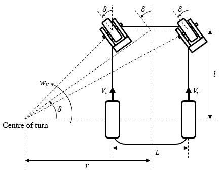
Since both rear wheels are driven by two motors, the speed of each driving wheel can be independently controlled. The electronic differential is therefore used to provide the required torques and speeds for each wheel. The slip on the rear wheels is ignored, so the speed of the wheels can be defined as a function of the radius of the wheels [21-23].
The Figure 2 shows the steering left of the FRE.
Figure 2. EPW design model during steering
The linear speed of each wheel drive can be expressed as:
$\left\{\begin{array}{l}V_{l}=w_{V}\left(r-\frac{L}{2}\right) \\ V_{r}=w_{V}\left(r+\frac{L}{2}\right)\end{array}\right.$ (7)
where, $r=\frac{l}{\tan \delta}$ and $\delta$ is the steering angle, the angular speeds are:
$\left\{\begin{array}{l}w_{l}=\frac{l-\left(\frac{L}{2}\right) \tan \delta}{l} w_{V} \\ w_{r}=\frac{l+\left(\frac{L}{2}\right) \tan \delta}{l} w_{V}\end{array}\right.$ (8)
If the steering angle $\delta>0$, the EPW drives left and if $\delta<0$, the EPW drives right. If $\delta=0$ , the EPW drives straight ahead.
$W_{V}$ is the centre of turn angular speed expressed by:
$w_{V}=\frac{w_{l}+w_{r}}{2}$ (9)
The backstepping is based on the second method of Lyapunov, which combine the choice of the energy function with the laws control. In addition to the task for which the controller is designed (tracking and/or regulation), this warranty at any time, the overall asymptotical stability of the compensated system.
Backstepping is a recursive procedure based on Lyapunov’s stability theory. Step by step, system states are chosen as virtual inputs to stabilize the corresponding subsystem [24].
One of the solutions to improve the robustness of the control by backstepping and to be able to eliminate the residual errors, in the presence of disturbances, is the introducing of an integral action in the controllers generated by the backstepping.
The steps of the control design are as follows:
Step 1: Control of right wheel position.
First, for right wheel position tracking objective defines the tracking error as:
$e_{1}=x_{1}-x_{1 r e f}+k_{x 1} \int_{0}^{t}\left(x_{1}-x_{1 r e f}\right) d t$ (10)
The Lyapunov law considered and it derivate are:
$V\left(e_{1}\right)=(1 / 2) e_{1}^{2}$ (11)
$\dot{V}\left(e_{1}\right)=e_{1}\left(\dot{x}_{1}-\dot{x}_{1 r e f}+k_{x 1}\left(x_{1}-x_{1 r e f}\right)\right)$ (12)
According to the state representation: .
To get the negative derivate of the Lyapunov function, the virtual control is considered as:
$x_{2}=\varphi\left(e_{1}\right)=-C_{1} e_{1}+\dot{x}_{1 r e f}-k_{x 1} x_{1}+k_{x 1} x_{1 r e f}$ (13)
Therefore: $\dot{V}\left(e_{1}\right)=-C_{1} e_{1}^{2}<0$ with $C_{1}>0$.
Since the theorem is verified; the first subsystem is asymptotically stable.
Step 2: Control of the right wheel speed.
For right wheel speed tracking objective defines the tracking error as:
$e_{2}=x_{2}-x_{2 r e f}+k_{x 2} \int_{0}^{t}\left(x_{2}-x_{2 r e f}\right) d t$ (14)
$x_{2 \text { ref }}$ is the previous virtual control $\varphi\left(e_{1}\right)$.
The increased energy function and it derivate are defined by:
$V\left(e_{1}, e_{2}\right)=1 / 2 e_{1}^{2}+1 / 2 e_{2}^{2}$ (15)
$\dot{V}\left(e_{1}, e_{2}\right)=e_{1} \dot{e}_{1}+e_{2} \dot{e}_{2}$ (16)
Development of $\dot{e}_{2}$:
$\begin{aligned} \dot{e}_{2}=\dot{x}_{2}-\dot{x}_{2 r e f} &+k_{x 2}\left(x_{2}-x_{2 r e f}\right) \\ &=l_{1} x_{2}+l_{2} x_{4}+y_{1} C e m_{r} \\ &+y_{2} C e m_{l}+T-\dot{x}_{2 r e f} \\ &+k_{x 2}\left(x_{2}-x_{2 r e f}\right) \end{aligned}$ (17)
The expression of $x_{2}$ ref and it derivate are:
$x_{2 r e f}=-C_{1} e_{1}+\dot{x}_{1 r e f}-k_{x 1}\left(x_{1}-x_{1 r e f}\right)$ (18)
$\begin{aligned} \dot{x}_{2 r e f}=-\left(k_{x 1}+\right.& \left.C_{1}\right)\left(e_{2}-x_{2 r e f}\right.\\ & \left.+k_{x 2} \int_{0}^{t}\left(x_{2}-x_{2 r e f}\right) d t\right) \\+& C_{1}\left(\dot{x}_{1 r e f}-k_{x 1}\left(x_{1}-x_{1 r e f}\right)\right) \end{aligned}$ (19)
Replacing in (12):
$\begin{aligned} \dot{e}_{2}=l_{1} x_{2}+l_{2} x_{4} &+y_{1} \mathrm{Cem}_{r}+y_{2} \mathrm{Cem}_{l}+T \\ &+k_{x 2}\left(x_{2}-x_{2 r e f}\right) \\ &+\left(k_{x 1}+C_{1}\right)\left(e_{2}-x_{2 r e f}\right.\\ & \left.+k_{x 2} \int_{0}^{t}\left(x_{2}-x_{2 r e f}\right) d t\right) \\ &-C_{1}\left(\dot{x}_{1 r e f}-k_{x 1}\left(x_{1}-x_{1 r e f}\right)\right) \end{aligned}$ (20)
The torque control expression is obtained:
$\begin{aligned} y_{1} \mathrm{Cem}_{r r e f}+y_{2} \mathrm{Cem}_{\text {lref }} \\ &=-C_{2} e_{2}-l_{1} x_{2}-l_{2} x_{4}-T \\ &-k_{x 2}\left(x_{2}-x_{2 r e f}\right) \\ &-\left(k_{x 1}+C_{1}\right)\left(e_{2}-x_{2 r e f}\right.\\ & \left.+k_{x 2} \int_{0}^{t}\left(x_{2}-x_{2 r e f}\right) d t\right) \\ &+C_{1}\left(\dot{x}_{1 r e f}-k_{x 1}\left(x_{1}-x_{1 r e f}\right)\right) \end{aligned}$ (21)
We note:
$\begin{aligned} y_{0}=-C_{2} e_{2}-l_{1} x_{2} &-l_{2} x_{4}-T-k_{x 2}\left(x_{2}-x_{2 r e f}\right) \\-&\left(k_{x 1}+C_{1}\right)\left(e_{2}-x_{2 r e f}\right.\\+& \left.k_{x 2} \int_{0}^{t}\left(x_{2}-x_{2 r e f}\right) d t\right) \\+& C_{1}\left(\dot{x}_{1 \text { ref }}-k_{x 1}\left(x_{1}-x_{1 r e f}\right)\right) \end{aligned}$ (22)
Thus: $\dot{V}\left(e_{1}, e_{2}\right)=-C_{1} e_{1}^{2}-C_{2} e_{2}^{2}<0$ with: $C_{1,2}>0$.
The stability of the two subsystems is checked.
To solve (21) with two unknown virtual inputs; another equation of the two torques will be made from the step 3 and 4.
Step 3: Control of left wheel position.
The tracking error is defined as:
$e_{3}=x_{3}-x_{3 r e f}+k_{x 3} \int_{0}^{t}\left(x_{3}-x_{3 r e f}\right) d t$ (23)
The augmented Lyapunov law and it derivate are:
$V\left(e_{1}, e_{2}, e_{3}\right)=\frac{1}{2} e_{1}^{2}+\frac{1}{2} e_{2}^{2}+\frac{1}{2} e_{3}^{2}$ (24)
$\dot{V}\left(e_{1}, e_{2}, e_{3}\right)=e_{1} \dot{e}_{1}+e_{2} \dot{e}_{2}+e_{3} \dot{e}_{3}$ (25)
According to the state representation: $\dot{x}_{3}=x_{4}$.
The virtual control is setting as:
$x_{4}=\varphi\left(e_{3}\right)=-C_{3} e_{3}+\dot{x}_{3 r e f}-k_{x 3} x_{3}+k_{x 3} x_{3 r e f}$ (26)
Therefore: $\dot{V}\left(e_{1}, e_{2}, e_{3}\right)=-C_{1} e_{1}^{2}-C_{2} e_{2}^{2}-C_{3} e_{3}^{2}<0$ with: $C_{1,2,3}>0$.
The stability of the increased systems is verified.
Step 4: Control of the left wheel speed.
For left wheel speed tracking objective defines the tracking error as:
$e_{4}=x_{4}-x_{4 r e f}+k_{x 4} \int_{0}^{t}\left(x_{4}-x_{4 r e f}\right) d t$ (27)
$x_{4 r e f}$ is the previous virtual control $\varphi\left(e_{3}\right)$.
Finally, the augmented Lyapunov law and it derivate are defined by:
$V\left(e_{1}, e_{2}, e_{3}, e_{4}\right)=\frac{1}{2} e_{1}^{2}+\frac{1}{2} e_{2}^{2}+\frac{1}{2} e_{3}^{2}+\frac{1}{2} e_{4}^{2}$ (28)
$\dot{V}\left(e_{1}, e_{2}, e_{3}, e_{4}\right)=e_{1} \dot{e}_{1}+e_{2} \dot{e}_{2}+e_{3} \dot{e}_{3}+e_{4} \dot{e}_{4}$ (29)
Development of $\dot{e}_{4}$:
$\begin{aligned} \dot{e}_{4}=\dot{x}_{4}-\dot{x}_{4 r e f}=& l_{3} x_{2}+l_{4} x_{4}+y_{3} C e m_{r} \\ &+y_{4} \text { Cem }_{l}+T+k_{x 4}\left(x_{4}-x_{4 r e f}\right) \\ &+\left(k_{x 3}+C_{3}\right)\left(e_{4}-x_{4 r e f}\right.\\ & \left.+k_{x 4} \int_{0}^{t}\left(x_{4}-x_{4 r e f}\right) d t\right) \\ &-C_{3}\left(\dot{x}_{3 r e f}-k_{x 3}\left(x_{3}-x_{3 r e f}\right)\right) \end{aligned}$ (30)
The torques control expression are:
$y_{3} \mathrm{Cem}_{\text {rref }}+y_{4}$ Cem $_{\text {lref }}$$=-C_{4} e_{4}-l_{3} x_{2}-l_{4} x_{4}-T$$\quad-k_{x 4}\left(x_{4}-x_{4 r e f}\right)$$\quad-\left(k_{x 3}+C_{3}\right)\left(e_{4}-x_{4 r e f}\right.$$\left.+k_{x 4} \int_{0}^{t}\left(x_{4}-x_{4 r e f}\right) d t\right)$$+C_{3}\left(\dot{x}_{3 r e f}-k_{x 3}\left(x_{3}-x_{3 r e f}\right)\right)$ (31)
We note:
$y_{5}=-C_{4} e_{4}-l_{3} x_{2}-l_{4} x_{4}-T-k_{x 4}\left(x_{4}-x_{4 r e f}\right)$$-\left(k_{x 3}+C_{3}\right)\left(e_{4}-x_{4 r e f}\right.$$\left.+k_{x 4} \int_{0}^{t}\left(x_{4}-x_{4 r e f}\right) d t\right)$$+C_{3}\left(\dot{x}_{3 r e f}-k_{x 3}\left(x_{3}-x_{3 r e f}\right)\right)$ (32)
Consequently: $\dot{V}\left(e_{1}, e_{2}, e_{3}, e_{4}\right)=-C_{1} e_{1}^{2}-C_{2} e_{2}^{2}-C_{3} e_{3}^{2}-$$C_{4} e_{4}^{2}<0$ with $C_{1,2,3,4}>0$.
The unknown control system is summarized as follow:
$\left\{\begin{array}{l}y_{1} \mathrm{Cem}_{\text {rref }}+y_{2} \mathrm{Cem}_{\text {lref }}=y_{0} \\ y_{3} \text { Cem }_{\text {rref }}+y_{4} \text { Cem }_{\text {lref }}=y_{5}\end{array}\right.$ (33)
The input right and left references torques is obtained after the resolution of the two last equations as:
Cem $_{\text {rref }}=y_{0} / y_{1}-y_{2} / y_{1}$ Cem $_{\text {lref }}$ (34)
Cem $_{\text {lref }}=y_{1} y_{5}-y_{3} y_{0} / y_{4} y_{1}-y_{3} y_{2}$ (35)
Step 5: Electromagnetic torque control of the right wheel.
For this step the error is:
$e_{5}=\mathrm{Cem}_{r}-\mathrm{Cem}_{r r e f}$$\quad+k_{x 5} \int_{0}^{t}\left(\mathrm{Cem}_{r}-\mathrm{Cem}_{r r e f}\right) d t$ (36)
The Lyapunov law considered and it derivate are:
$V\left(e_{1}, e_{2}, e_{3}, e_{4}, e_{5}\right)$$=\frac{1}{2} e_{1}^{2}+\frac{1}{2} e_{2}^{2}+\frac{1}{2} e_{3}^{2}+\frac{1}{2} e_{4}^{2}$$+\frac{1}{2} e_{5}^{2}$ (37)
$\dot{V}\left(e_{1}, e_{2}, e_{3}, e_{4}, e_{5}\right)$$=e_{1} \dot{e}_{1}+e_{2} \dot{e}_{2}+e_{3} \dot{e}_{3}+e_{4} \dot{e}_{4}$$+e_{5} \dot{e}_{5}$ (38)
Development of $\dot{e}_{5}$:
$\dot{e}_{5}=\dot{{Cem}}_{r}-\dot{{Cem}}_{{rref }}+k_{x 5}\left({Cem}_{r}-{Cem}_{ {rref }}\right)$ (39)
The torque expression (rotor surface magnets) is defined as:
${Cem}_{r}=P \varphi_{f} I_{q r}$ (40)
Replacing (40) in (39):
$\dot{e}_{5}=P \varphi_{f} / L_{d}\left[\left(V_{q r}-R_{s} I_{q}-w L_{d} I_{q}-w \varphi_{f}\right)\right.$$\dot{Cem}\left._{ {rref }}\right]$$+k_{x 5}\left({Cem}_{r}-{Cem}_{r r e f}\right)$ (41)
The real input control of the right motor is:
$V_{q r}=-C_{5} e_{5}+R_{s} I_{q}+w L_{d} I_{d}+w \varphi_{f}$$+L_{q} / P \varphi_{f}\dot{Cem}_{{rref }}$$-L_{q} / P \varphi_{f}\left(k_{x 5}\left(\mathrm{Cem}_{r}\right.\right.$$-$ Cem $\left._{\text {rref }}\right)$ ) (42)
With:
$\dot{Cem}_{ {rref }}=\left(1 / y_{0}\right) \dot{y}_{0}-\left(y_{2} / y_{1}\right)\dot{Cem}_{ {lref }}$ (43)
And:
$\dot{y}_{0}=-\left[\left(C_{2}+C_{1}+k_{x 1}+k_{x 2}+l_{1}\right) l_{1}\right.$$+\left(C_{2}+C_{1}+k_{x 1}-C_{1}\right.$$\left.-k_{x 1}\right) k_{x 2}+l_{2} l_{3}$
$\left.+C_{1} k_{x 1}\left(C_{1}+k_{x 1}\right)\right] x_{2}$$-\left[\left(C_{2}+C_{1}+k_{x 2}+l_{1}\right.\right.$$\left.\left.+k_{x 2}+l_{4}\right) l_{2}\right] x_{4}$
$-\left[\left(C_{2}+C_{1}+k_{x 1}+l_{1}+k_{x 2}\right) y_{1}\right.$$\left.+y_{3} l_{2}\right] \mathrm{Cem}_{\text {rref }}$$-\left[\left(l_{2}+l_{1}+k_{x 2}\right) y_{4}\right.$$\left.+\left(C_{2}+C_{1}+k_{x 1}\right) y_{2}\right] C e m_{\text {lref }}$ (44)
$-\left[C_{2}+C_{1}+k_{x 1}+l_{1}+k_{x 2}+l_{2}\right] T$$+\left[\left(C_{2}+C_{1}+k_{x 1}\right)\left(C_{1}+k_{x 2}\right.\right.$$\left.\left.+k_{x 1}\right)+\left(C_{1}+k_{x 1}\right) k_{x 2}\right] x_{4 r e f}$
$-\left[\left(C_{2}+C_{1}+k_{x 1}\right)\left(C_{1}+k_{x 1}\right)\right] e_{4}$$-\left(C_{2}+C_{1}+k_{x 1}\right)\left(C_{1}\right.$$\left.+k_{x 1}\right) k_{x 2} \int_{0}^{l}\left(x_{2}-x_{2 r e f}\right) d t$
$-C_{1} k_{x 1}\left(C_{2}+C_{1}+k_{x 1}\right)\left(x_{1}\right.$$\left.-x_{1 \text { ref }}\right)$
Therefore: $\dot{V}\left(e_{1}, e_{2}, e_{3}, e_{4}\right)=-C_{1} e_{1}^{2}-C_{2} e_{2}^{2}-C_{3} e_{3}^{2}-$$C_{4} e_{4}^{2}<0$ with $C_{1,2,3,4}>0$.
Step 6: Control of the left wheel torque.
Take $e_{6}$ as last error:
$e_{6}=\mathrm{Cem}_{l}-\mathrm{Cem}_{\text {lref }}$$+k_{x 6} \int_{0}^{t}\left(C e m_{l}-C e m_{l r e f}\right) d t$ (45)
The last Lyapunov increased function and it derivate are:
$V\left(e_{1}, e_{2}, e_{3}, e_{4}, e_{5}, e_{6}\right)$$=\frac{1}{2} e_{1}^{2}+\frac{1}{2} e_{2}^{2}+\frac{1}{2} e_{3}^{2}+\frac{1}{2} e_{4}^{2}$$+\frac{1}{2} e_{5}^{2}+\frac{1}{2} e_{6}^{2}$ (46)
$\dot{V}\left(e_{1}, e_{2}, e_{3}, e_{4}, e_{5}, e_{6}\right)$$=e_{1} \dot{e}_{1}+e_{2} \dot{e}_{2}+e_{3} \dot{e}_{3}+e_{4} \dot{e}_{4}$$+e_{5} \dot{e}_{5}+e_{6} \dot{e}_{6}$ (47)
Development of $\dot{e}_{6}$:
$\dot{e}_{6}=\dot{Cem}_{l}-\dot{ { Cem }_{{lref }}}+k_{x 6}\left(\right.$ Cem $_{l}-$ Cem $\left._{ {lref }}\right)$ (48)
The torque expression:
$\operatorname{Cem}_{l}=P \varphi_{f} I_{q l}$ (49)
Replacing (49) in (48):
$\dot{e}_{6}=P \varphi_{f} / L_{d}\left[\left(V_{q l}-R_{s} I_{q}-w L_{d} I_{q}-w \varphi_{f}\right)\right.$$\left.-C \dot{e} m_{\text {lref }}\right]$$+k_{x 6}\left(\mathrm{Cem}_{l}-\mathrm{Cem}_{\text {lref }}\right)$ (50)
The real input control:
$V_{q l}=-C_{6} e_{6}+R_{s} I_{q}+w L_{d} I_{d}+w \varphi_{f}$$+L_{q} / P \varphi_{f}\dot{Cem}_{{lref }}$$-L_{q} / P \varphi_{f}\left(k_{x 6}\left({Cem}_{l}\right.\right.$$-cem_{ {lref }}))$ (51)
With:
$\dot{Cem}_{ {rref }}=\left(1 / y_{4} y_{1}-y_{3} y_{2}\right)\left(y_{1} \dot{y}_{5}-y_{3} \dot{y}_{0}\right)$ (52)
And:
$\dot{y}_{5}=-\left[\left(C_{3}+C_{4}+k_{x 3}+l_{1}+k_{x 4}+l_{4}\right) l_{3}\right] x_{2}$$-\left[\left(C_{3}+C_{4}+k_{x 3}+k_{x 4}+l_{4}\right) l_{4}\right.$
$+\left(C_{3}+C_{4}+k_{x 3}-C_{3}-k_{x 3}\right) k_{x 4}$$\left.+l_{2} l_{3}+C_{3} k_{x 3}\left(C_{3}+k_{x 3}\right)\right] x_{4}$$-\left[\left(C_{3}+C_{4}+k_{x 3}+l_{4}+k_{x 4}\right) y_{3}\right.$$\left.+y_{1} l_{3}\right]$ Cem $_{ {rref }}$
$-\left[\left(C_{3}+C_{4}+k_{x 3}+l_{4}+k_{x 4}\right) y_{4}\right.$$\left.+y_{2} l_{3}\right]$ Cem $_{ {lref }}$$-\left[C_{3}+C_{4}+k_{x 3}+l_{4}+k_{x 4}+l_{3}\right] T$ (53)
$+\left[\left(C_{3}+C_{4}+k_{x 3}\right)\left(C_{3}+k_{x 4}\right.\right.$$\left.\left.+k_{x 3}\right)+\left(C_{3}+k_{x 3}\right) k_{x 4}\right] x_{{ 4ref }}$$-\left[\left(C_{3}+C_{4}+k_{x 3}\right)\left(C_{3}+k_{x 3}\right)\right] e_{4}$
$-\left(C_{3}+C_{4}+k_{x 3}\right)\left(C_{3}\right.$$\left.+k_{x 3}\right) k_{x 4} \int_{0}^{t}\left(x_{4}-x_{4 r e f}\right) d t$$-C_{3} k_{x 3}\left(C_{3}+C_{4}+k_{x 3}\right)\left(x_{3}\right.$$\left.-x_{3 { ref }}\right)$
Therefore: $\dot{V}\left(e_{1}, e_{2}, e_{3}, e_{4}, e_{5}, e_{6}\right)=-C_{1} e_{1}^{2}-C_{2} e_{2}^{2}-$$C_{3} e_{3}^{2}-C_{4} e_{4}^{2}-C_{5} e_{5}^{2}-C_{6} e_{6}^{2}<0$ with: $C_{1,2,3,4,5,6}>0$.
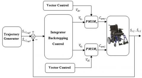
The block diagram for the IBC application on the EPW is illustrated in Figure 3.
Figure 3. Block diagram of the IBC for EPW
Figure 4. Structure of the FLC
As shown in Figure 4, the FLC structure has three main components such as fuzzification, fuzzy inference engine (decision logic), and defuzzification [11].
The first block is fuzzification which converts each element of input data to degrees of membership by a lookup in one or several membership functions. The rule base and inference base have the capability of simulating human decision-making based on fuzzy concepts and the capability of inferring fuzzy control actions employing fuzzy implication and the rules of inference in fuzzy logic. The third operation is called as defuzzification. The resulting fuzzy set is defuzzified into a crisp control signal. The most common methods are as follows: Center of Gravity (COG), Bisector of Area (BOA), Mean of Maximum (MOM), Smallest of Maximum (SOM) and Largest of Maximum (LOM) [25, 26].
The designing procedure of the fuzzy controller [12] applied to EPW is described as follows:
Step 1. Choice of inputs and outputs of FLC: The input variables of the FLC are error, e ( $e_{r}=S_{r_{r e f}}-S_{r}$ and $e_{l}=S_{l_{r e f}}-S_{l}$) and error derivation, $\dot{e}$ of wheel position. The output variable of the fuzzy controller is the driving wheel control input $V_{q}$.
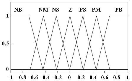
Step 2. Definition of membership functions of FLC: Each input and output variable have seven fuzzy sets. The triangular and trapezoidal membership functions were used for both input and output of FLC to the interval [-1, 1], as shown in Figure 5 and Figure 6.
Figure 5. Membership functions of input $e_{r}, \dot{e}_{r}, e_{l}, \dot{e}_{l}$
Figure 6. Membership functions of output $V_{q r}, V_{q l}$
Note: The abbreviations used in the figure mean: NB (Negative Big), NM (Negative Medium), NS (Negative Small), Z (Zero), PS (Positive Small), PM (Positive Medium) and PB (Positive Big).
Step 3. Design of the inference mechanism rules to find the input-output relation: This paper uses Mamdani (Max-Min) inference mechanism. The fuzzy IF-THEN rules of the controller are given in Table 2.
Step 4. Defuzzification of the output variable of fuzzy mechanism: The resulting fuzzy set must be converted to a signal that can be sent to the process as a control input. Center of gravity was used here for defuzzification schema.
Table 2. Rule base of EPW
|
e $\dot{e}$ |
NB |
NM |
NS |
Z |
PS |
PM |
PB |
|
NB |
NB |
NB |
NM |
NM |
NS |
NS |
Z |
|
NM |
NB |
NM |
NM |
NS |
NS |
Z |
PS |
|
NS |
NM |
NM |
NS |
NS |
Z |
PS |
PS |
|
Z |
NM |
NS |
NS |
Z |
PS |
PS |
PM |
|
PS |
NS |
NS |
Z |
PS |
PS |
PM |
PM |
|
PM |
NS |
Z |
PS |
PS |
PM |
PM |
PB |
|
PB |
Z |
PS |
PS |
PM |
PM |
PB |
PB |
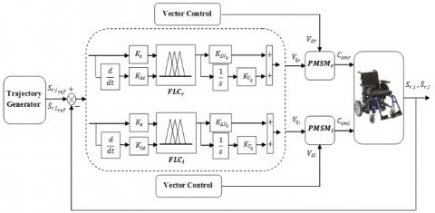
The block diagram for the FLC application on the EPW is illustrated in Figure 7.
Figure 7. Block diagram of the FLC for EPW
To evaluate the performance of the two controls applied to EPW driven by two PMSM, we simulate the displacement and velocity tracking, we also show the evolution of electrical and mechanical quantities.
First, we start by generating the reference movements of the right and left wheel. The use of polynomial form is a very practical tool for calculating movement. The most frequently encountered polynomial interpolation method is interpolation by the fifth-degree polynomials, which ensures the continuity of movement in position, velocity and acceleration [27, 28].
The point-to-point trajectory between $S^{i}$ and $S^{f}$ is determined by the following equations:
$S(t)=S^{i}+r(t) D$ for $0 \leq t \leq t_{f}$ (54)
$\dot{S}(t)=\dot{r}(t) \mathrm{D}$ (55)
With: $D=S^{f}-S^{i}$. the values at the limits of the interpolation function $r(t)$ are given by: $r(0)=0$ and $r(t f)=1$.
The polynomial is obtained by using the following boundary conditions: $S(0)=S^{i}$, $S\left(t_{f}\right)=S^{f}$, $\dot{S}(0)=0$, $\dot{S}\left(t_{f}\right)=0$, $\ddot{S}(0)=0$, $\ddot{S}\left(t_{f}\right)=0$.
And, using the following polynomial form:
$S(t)=a_{0}+a_{1} t+a_{2} t^{2}+a_{3} t^{3}+a_{4} t^{4}+a_{5} t^{5}$ (56)
We show that the movement function of the fifth-degree can be in the form (54) or (55) with:
$r(t)=10\left(\frac{t}{t_{f}}\right)^{3}-15\left(\frac{t}{t_{f}}\right)^{4}+6\left(\frac{t}{t_{f}}\right)^{5}$ (57)
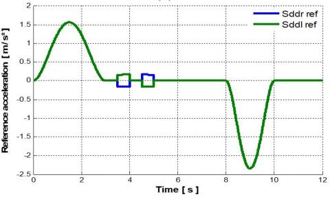
(a)
(b)
(c)
Figure 8. Reference trajectories of the right/left wheel. (a) Displacement, (b) Velocity, (c) Acceleration
Table 3. Parameters IBC
|
Parameter |
Value |
|
C1=C3 |
1000 |
|
C2=C4 |
10 |
|
Kx1=kx3 |
1000 |
|
Kx2=kx4 |
500 |
Table 4. Parameters FLC
|
Parameter |
Value |
|
$k_{e r}=k_{e l}$ |
500 |
|
$k_{\Delta e r}=k_{\Delta e l}$ |
100 |
|
$K_{V_{q r}}=K_{V_{q l}}$ |
400 |
|
$K_{\Delta V_{q r}}=K_{\Delta V_{q l}}$ |
5000 |
For a displacement of 0 m to 18.75 m in 10 s which correspond to a variable velocity up to 2.5 m/s, we have opted for the trajectories shown in Figure 8 by performing a slope variation from $\psi=0 \%$ to $\psi=0.17 \%$ in the time interval t=5.5 s to t=7.5 s and a direction change from $\delta=0^{\circ}$ to $\delta=0.1^{\circ}$ between t=3.5 s and t=5 s achieved by the electronic differential. During this turning, the wheels don’t turn at the same velocity. Indeed, the left wheel travels more distance than the right wheel.
After several simulation tests by using the method of trial and error for each controller, we obtain the adequate parameters in Table 3 and Table 4.
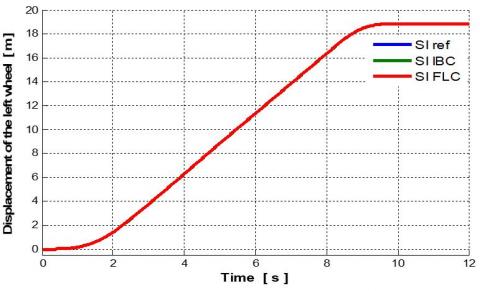
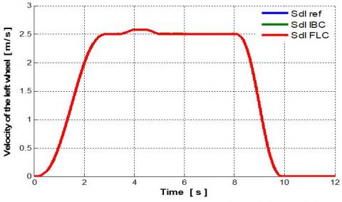
Figure 9, Figure 10, Figure 11 and Figure 12 represent, respectively the displacement and velocity trajectory tracking of the right and left drive wheel, we note that the measured trajectories perfectly follow the references. The velocities increase to a maximum value which remains maintained during the steady state and then returns to zero, which corresponds to the final state.
Figure 9. Displacement of the right wheel
Figure 10. Displacement of the left wheel
Figure 11. Velocity of the right wheel
Figure 12. Velocity of the left wheel
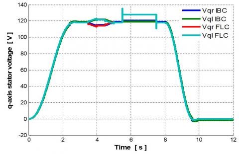
Figure 13 shows the evolution of the electromagnetic torque $C_{e m r, l}$ of the both PMSM, they increase to a maximum value, then they return to a very small positive value which remains constant in steady state, however, they react in the case of turning and slope variation, then they go to a negative minimum value and return to zero at the end. These torques are directly proportional to the stator quadrature currents $I_{q r, l}$ given in Figure 14. The stator direct currents $I_{d r, l}$ are maintained at zero by the vector control as shown in Figure 15. The direct and quadrature voltage inputs of both PMSM $\left(V_{d r, l}, V_{q r, l}\right)$ don’t exceed their nominal values as shown in Figure 16 and Figure 17 respectively. Likewise, the steering left and slope variation have no effect on the various quantities of the system.
The results obtained show the efficiency of the two controls of the global system (EPW+PMSM), with better tracking, fast response, without overshoot.
Figure 13. Electromagnetic torque of the right/ left motor
Figure 14. q-axis stator current of the right/left motor
Figure 15. d-axis stator current of the right/ left motor
Figure 16. d-axis stator voltage of the right/ left motor
Figure 17. q-axis stator voltage of the right/ left motor
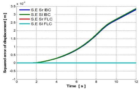
Figure 18. Squared error of displacement
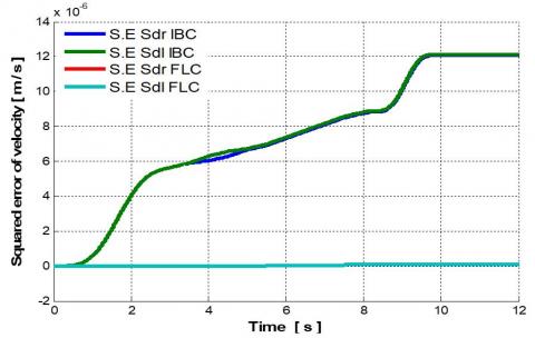
Figure 19. Squared error of velocity
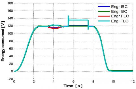
Figure 20. Energy consumed
To compare the performance of these two controls, we performed two measurements. The first is to plot the evolution of the squared error of the displacement and velocity during the application of the different commands shown in Figure 18 and Figure 19 respectively, while the second measure will allow the plot of the evolution of the energy consumed as shown in Figure 20. Comparing squared errors, we find that fuzzy control is even more accurate than the integral backstepping control because it has less error. While the energy consumed is almost the same for both controllers.
In this study, a dynamic modelling of EPW using PMSM as an actuator is considered. It is an electromechanical, multivariable, nonlinear and strongly coupled system, hence the necessity to introduce the robust controllers.
A nonlinear command by backstepping with integral action was applied to the model (EPW+PMSM) in the first. With this control, the quality of the performances in the static and dynamic states is ensured. Robustness intrinsic to backstepping is reinforced through the integral’s terms added in the design of the backstepping law. In the second half, the fuzzy logic controller was established to track the trajectory of the EPW. This technique, based on artificial intelligence, improves the precision and robustness of the controlled system.
The different results obtained confirm the feasibility of the two controllers with slight difference when applying the FLC.
An experimental implementation of these two controllers is targeted in future work.
[1] Geonea, I., Dumitru, N., Dumitru, V. (2015). Design and motion analysis of a powered wheelchair. Applied Mechanics and Materials, 772: 613-620. https://doi.org/10.4028/www.scientific.net/AMM.772.613
[2] Boubekeur, D., Boumédiène, A., Sari, Z., Tahraoui, S. (2015). Modeling and backstepping control for electric powered wheelchair. International Electrical and Computer Engineering Conference, Setif, Algeria.
[3] Velàzquez, R., Gutiérrez, C.A. (2014). Modeling and control techniques for Electric Powered Wheelchair: An Overview. IEEE Central America and Panama Convention (CONCAPAN XXXIV), pp. 1-6. https://doi.org/10.1109/CONCAPAN.2014.7000435
[4] Dou, X.X., Tong, Q.M. (2011). The application of permanent magnet electric machine on electrical wheelchair. Advanced Materials Research, 383-390: 7161-7165. https://doi.org/10.4028/www.scientific.net/AMR.383-390.7161
[5] Shimada, S., Ishimura, K., Wada, M. (2003). System design of electric wheelchair for realizing adaptive operation to human intention. IEEE International conference on Robotic, Intelligent systems and Signal Processing, pp. 513-518. https://doi.org/10.1109/RISSP.2003.1285627
[6] Boquete, L., Garcia, R., Berea, R., Maro, M. (1999). Neural control of the movements of a wheelchair. Journal of Intelligent and Robotic Systems, 25(3): 213-226. https://doi.org/10.1023/A:1008068322312
[7] Ma, J. (2014). Design on electric power wheel control system. Advanced Materials Research, 1070-1072: 1668-1671. https://doi.org/10.4028/www.scientific.net/AMR.1070-1072.1668
[8] Yang, F.Y., Tsai, M.C. (2012). Synchronous decoupled motion control for power-wheelchairs. Advanced Materials Research, 482-484: 1904-1911. https://doi.org/10.4028/www.scientific.net/AMR.482-484.1904
[9] Nguyen, T.N., Su, S.W., Nguyen, H.T. (2011). Robust neuro-sliding mode multivariable control strategy for powered wheelchairs. IEEE Transactions on Neural Systems and Rehabilitation Engineering, 19(1): 105-111. https://doi.org/10.1109/TNSRE.2010.2069104
[10] Ayten, K.K., Dumlu, A., Kaleli, A. (2017). Real-time trajectory tracking control for electric-powered wheelchairs using model-based multivariable sliding mode control. 5th International Symposium on Electrical and Electronics Engineering, pp. 1-6. https://doi.org/10.1109/ISEEE.2017.8170636
[11] Bingül, Z., Karahan, O. (2011). A Fuzzy Logic Controller tuned with PSO for 2 DOF robot trajectory control. Expert Systems with Applications, 38(1): 1017-1031. https://doi.org/10.1016/j.eswa.2010.07.131
[12] Kharidege, A., Ding, J.B., Zhang, Y.J. (2016). Performance study of PID and fuzzy controllers for position control of 6 DOF arm manipulator with various defuzzification strategies. 3rd International Conference on Mechanics and Mechatronics Research, 77: 01011. https://doi.org/10.1051/matecconf/20167701011
[13] Rojas, M., Ponce, P., Molina, A. (2018). A fuzzy logic navigation controller implemented in hardware for an electric wheelchair. International Journal of Advanced Robotic Systems, 15(1). https://doi.org/10.1177/1729881418755768
[14] Barriuso, A.L., Pérez-Marcos, J., Jiménez-Bravo, D.M., González, G.V., De Paz, J.F. (2018). Agent-based intelligent interface for Wheelchair Movement Control. Sensors, 18(5): 1511. https://doi.org/10.3390/s18051511
[15] Jamin, N.F., Ghani, N.M.A., Ibrahim, Z., Masrom, M.F., Razali, N.A.A., Almeshal, A.M. (2018). Two-wheeled wheelchair stabilization using Interval Type-2 Fuzzy Logic Controller. International Journal of Simulation: Systems, Science & Technology, 19(3): 3.1-3.7. https://doi.org/10.5013/IJSSST.a.19.03.03
[16] Maatoug, K., Njah, M., Jallouli, M. (2019). Electric wheelchair trajectory tracking control based on Fuzzy Logic Controller. 19th International Conference on Sciences and Techniques of Automatic Control and Computer Engineering, pp. 191-195. https://doi.org/10.1109/STA.2019.8717190
[17] Dadios, E.P. (2012). Fuzzy Logic - Controls, Concepts, Theories and Applications. InTechOpen, UK. https://doi.org/10.5772/2662
[18] Mecifi, M., Boumédiène, A., Boubekeur, D. (2019). A fuzzy logic controller for electric powered wheelchair based on Lagrange model. International Conference on Advanced Electrical Engineering, pp. 1-6. https://doi.org/10.1109/ICAEE47123.2019.9014838
[19] Herrera, D., Roberti, F., Carelli, R., Andaluz, V., Varela, J., Ortiz, J., Canseco, P. (2018). Modeling and path-following control of a wheelchair in human-shared environments. International Journal of Humanoid Robotics, 15(2): 1850010. https://doi.org/10.1142/S021984361850010X
[20] Dhaouadi, R., Hatab, A.A. (2013). Dynamic modelling of differential-drive mobile robots using Lagrange and Newton-Euler Methodologies: A unified framework. Advances in Robotics and Automation, 2(2): 107. https://doi.org/10.4172/2168-9695.1000107
[21] Aggarwal, A. (2013). Electronic differential in electric vehicles. International Journal of Scientific & Engineering Research, 4(11).
[22] Ozkop, E., Altas, I.H., Okumus, H.I., Sharaf, A.M. (2015). A fuzzy logic sliding mode controlled electronic differential for a direct wheel drive EV. International Journal of Electronics, 102(11): 1919-1942. https://doi.org/10.1080/00207217.2015.1010183
[23] Tsai, M.C., Wu, K.S., Hsueh, P.W. (2009). Synchronized motion control for power-wheelchairs. Fourth International Conference on Innovative Computing, Information and Control, Kaohsiung, Taiwan, pp. 908-913. https://doi.org/10.1109/ICICIC.2009.344
[24] Shim, H.M., Hong, J.P., Chung, S.B., Hong, S.H. (2001). A powered wheelchair controller based on master-slave control architecture. IEEE International Symposium on Industrial Electronics Proceedings (Cat. No.01TH8570), 3, Pusan, Korea (South), 3: 1553-1556. https://doi.org/10.1109/ISIE.2001.931937
[25] Talon, A., Curt, C. (2017). Selection of appropriate defuzzification methods: Application to the assessment of dam performance. Expert Systems with Applications, 70: 160-174. https://doi.org/10.1016/j.eswa.2016.09.004
[26] Mogharreban, N., Dilalla, L. (2006). Comparison of defuzzification techniques for analysis of non-interval data. Annual Meeting of the North American Fuzzy Information Processing Society, Montreal, QC, Canada, pp. 257-260. https://doi.org/10.1109/NAFIPS.2006.365418
[27] Dombre, E., Khalil, W. (2007). Modeling, Performance Analysis and Control of Robot Manipulators. Wiley-ISTE. https://doi.org/10.1002/9780470612286
[28] Mohammed, M.Q., Miskon, M.F., Bahar, M.B., Ali, S.A. (2017). Comparative study between quintic and cubic polynomial equations based walking trajectory of exoskeleton system. International Journal of Mechanical & Mechatronics Engineering, 17(4): 43-51.