Li Zhang* | Yiming Sun | Shuning Cai | Jianing Yuan | Boyi Wang
© 2020 IIETA. This article is published by IIETA and is licensed under the CC BY 4.0 license (http://creativecommons.org/licenses/by/4.0/).
OPEN ACCESS
Drawing on the principles of non-intrusive load monitoring (NILM) and the load parameter detection function of smart remote load controller (SRLC), this paper presents a non-intrusive load identification method based on real-time extraction of multiple steady-state parameters and the optimization of state coding. Firstly, the characteristic parameters of loads were extracted by the Intelligent Power Management Platform, and the original load data were clustered by the improved affinity propagation (AP) algorithm, creating a sample set of multiple steady-state parameters. Considering the working states of loads, a load decomposition model was established, and the objective function was optimized by genetic algorithm (GA), realizing the decomposition and re-identification of household loads. Finally, our method was proved to have an accuracy of over 96% through experiments. The research results provide a reference for electricity department to identify the type and features of loads on the consumer side.
non-intrusive load monitoring (NILM), load identification, steady-state parameters, affinity propagation (AP) clustering
In demand-side management (DSM), the growth in power consumption has widened the peak-to-valley difference of the grid, pushing up the demand for load regulation on consumer side. The variety of load types, coupled with the ever-changing power demand, directly bear on the operation state of the entire power regulation system. This calls for active response and flexible regulation of user terminal load. For this purpose, it is necessary to probe deep into the consumption features and information of loads, laying the basis for effective load identification [1, 2].
Load identification is inseparable from load monitoring. The two main load monitoring methods are intrusive load monitoring (ILM) and non-intrusive load monitoring (NILM). Currently, NILM has replaced ILM as the mainstream approach, thanks to its low cost, simple communication, and ease of maintenance and promotion [3, 4]. The essence of NILM is load decomposition. Owing to the sheer number of users and complex structure of load system, the key difficulty of NILM is to effectively decompose load type from the total load and identify the load state.
Over the past decade, many scholars have explored deep into load identification based on NILM. For instance, Liang et al. [5] recognized the working and non-working states of each load by committee decision mechanisms (CDMs), and proved that the CDMs outperforms load identification methods based on single feature or single algorithm. Using heuristic algorithm and Bayesian classifier, Marchiori et al. [6] conducted non-intrusive load identification based on steady-state power and step change of loads. Chang et al. [7] combined neural network (NN) and wavelet transform (WT) into a load identification method, which effectively improves the speed of load identification, but some loads might not be detected if the wavelet basis function is improperly selected before the identification.
Considering the transient features of load power, Gao and Yang [8] identified loads by comparing the closeness of the data on load features; Based on high-frequency sampling, this load identification strategy has a high requirement on sampling and induces a huge workload of data analysis, both of which limit the application scope of the strategy. Abdullah-al-nahid et al. [9] improved Canny edge detection to recognize the pattern of low-power loads, but the improved method is slow in detecting edge mutations and not highly accurate. Qi et al. [10] developed an identification method for household loads based on Fisher’s supervised discrimination, and obtained the optimal identification features by reducing the dimensionality of characteristic load samples from eight typical electrical appliances; Nevertheless, the identification accuracy of their method depends heavily on the accuracy of sample classification.
Yang et al. [11] put forward a load identification method that fuses feature sequences; On average, the load accuracy and identification accuracy of this method are both above 90.8%; But the high accuracy is achieved at the cost of a long time and heavy computing load. Wang et al. [12] created an NILM algorithm based on voltage-current (V-I) trajectory: The V-I trajectory increment was extracted through interpolation, and the loads were identified accurately with the aid of support vector machine (SVM). In 2019, Welikala et al. [13] designed a novel NILM approach that actively identifies real-time loads in view of appliance usage patterns (AUPs), shedding new light on load identification amidst massive load monitoring data.
The above non-intrusive load identification methods each has its merits and defects. During implementation, every method is limited by some conditions. If some conditions are not satisfied, it is difficult to create a highly accurate model by the method, making the method unpromotable in practice. To solve the problem, this paper presents a non-intrusive load identification method based on real-time extraction of multiple steady-state parameters and the optimization of state coding. Specifically, the improved affinity propagation (AP) algorithm was adopted to cluster the original load data, and construct a sample set of load power characteristic parameters. A load decomposition model was established, and the objective function was optimized by genetic algorithm (GA), facilitating the decomposition and re-identification of household loads. Empirical results show that our method achieved an accuracy above 96%. Our method applies to load identification against massive data. It is widely applicable, and easy to popularize. The research results provide a technical reference for non-intrusive identification of household loads.
With the rising standard of living, there is a growing demand for household appliances. The household loads differ greatly in type, functions, and steady state. The power waveforms and load data of 30 most used household appliances in China (Table 1) were observed for a long period. Based on the observed data, the household loads were divided into three categories: 0-1 state equipment (ON/OFF) (Category I), finite-state machines (FSM) (Category II), and continuously variable devices (CVD) (Category III) [14].
Table 1. Thirty electrical appliances commonly used by residents
|
No. |
Name |
Rated power |
No. |
Name |
Rated power |
|
1 |
Cabinet air conditioner |
3,000/4,000W (Cool/ Hot) |
16 |
Refrigerator |
115W |
|
2 |
Split air conditioner |
1,900/2,300W (Cool/ Hot) |
17 |
Electric rice cooker |
450W |
|
3 |
Television (TV) |
105W |
18 |
Induction cooker |
3,000W |
|
4 |
Electric kettle |
1,600W |
19 |
Microwave oven |
1,500W |
|
5 |
Hair drier |
1,200W |
20 |
Range hood |
200W |
|
6 |
Heater fan |
1,300W |
21 |
Electric oven |
1,600W |
|
7 |
Water dispenser |
1,400W |
22 |
Soybean milk machine |
1,200W |
|
8 |
Electric fan |
100W |
23 |
Electric baking pan |
1,450W |
|
9 |
Garment steamer |
1,800W |
24 |
Dishwasher |
1,150W |
|
10 |
Light-emitting diode (LED) light |
35W |
25 |
Juicer |
500W |
|
11 |
Multimode lamp |
110W |
26 |
Water heater |
3,000W |
|
12 |
Vacuum cleaner |
1,000W |
27 |
Washing machine |
320W |
|
13 |
Air cleaner |
50W |
28 |
Printer |
280W |
|
14 |
Electric blanket |
125W |
29 |
Laptop |
95W |
|
15 |
Electric heater |
2,200W |
30 |
Home audio |
250W |
Figure 1. Power waveform of Category I appliances
Category II: Finite-state machines have multiple working states (working modes / power ranges), but the number of states is generally not more than eight. During operation, the working mode changes with the consumption power, the load features are relatively stable and independent, and the power waveform is shaped like a step. As shown in Figure 2, the representative appliances in this category include electric oven, hair dryer, electric fan, etc.
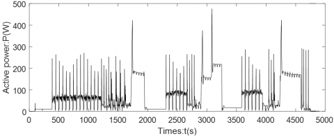
Category III: Continuously variable devices do not have stable steady-state features. During operation, the load changes continuously, and the power has high uncertainty, due to the lack of fixed working rules and procedures. The power varies greatly between adjacent working cycles. As shown in Figure 3, the power waveform is approximately a finite number of discrete states obtained through random observations. The typical appliances in this category include cabinet air conditioner and washing machine.
Figure 2. Power waveform of Category II appliances
Figure 3. Power waveform of Category III appliances
Residential households generally use resistive load appliances, most of which belong to Categories I and II. For these appliances, the active power is obvious, while the reactive power is extremely small. Besides, there is no significant transient process in the switching process. Thus, these appliances are linear loads, whose current or voltage waveform is stable and easy to detect and identify. Hence, active power was regarded as the main feature of the appliances in the two categories.
The appliances in Category III are mostly nonlinear loads with capacitive or inductive features. In nonlinear loads, the internal circuit contains nonlinear elements (e.g. capacitors, inductors, and motors) that might distort the current waveform [15]. There is a nonnegligible transient process in the switching process. Thus, reactive power was considered the main feature of Category III appliances.
For the above three types of loads, the power factor is an important parameter to distinguish between resistive, capacitive, and inductive loads. Through the above analysis, active power (P), reactive power (Q), and power factor (F) were taken as the steady-state parameters to be collected, according to the features of different types of appliances.
3.1 NILM system
As shown in Figure 4, our NILM system is designed based on smart remote load controller (SRLC). The SRLC is a product independently developed by our research team. Embedded with advanced sensors and processors, the SRLC-based system can monitor the operation and energy consumption of user loads online, and, in association with multi-function smart meters, to collect all load data, preprocess current and voltage signals, and extract and analyze characteristic load parameters. The collection of active power was taken as an example to illustrate the proposed NILM system.
Figure 4. The monitoring circuit of the SRLC-based NILM
Let L1, L2, L3, ..., LN be the power loads of a household. Then, the set of samples for load data acquisition L can be described as:
$L=({{L}_{1}},{{L}_{2}},{{L}_{3}},...{{L}_{N}})$ (1)
where, L1, L2, L3, ..., LN are vectors. The load data that correspond to the vectors can be respectively expressed as:
$\begin{align} & {{L}_{1}}(k)=\{{{l}_{1}}(0),{{l}_{1}}(1),...{{l}_{1}}(k)\}, \\ & {{L}_{2}}(k)=\{{{l}_{2}}(0),{{l}_{2}}(1),...{{l}_{2}}(k)\}, \\ & {{L}_{3}}(k)=\{{{l}_{3}}(0),{{l}_{3}}(1),...{{l}_{3}}(k)\}, \\ & ..., \\ & {{L}_{n}}(k)=\{{{l}_{N}}(0),{{l}_{N}}(1),...{{l}_{N}}(k)\} \\ \end{align}$ (2)
where, k is the number of sampling points; N is the total number of appliances; L1(k), L2(k), L3(k), ..., LN(k) are the active powers of the sampling points. The sets of samples for the acquisition of reactive power and power factor were acquired in a similar manner.
3.2 Load feature sequence
K-means clustering (KMC) and fuzzy C-means (FCM) clustering are two popular clustering methods. For both methods, the number of clusters must be configured rationally in advance. The subjective configuration will affect the clustering results. Besides, the clustering results will change with the initial cluster center. Therefore, it is necessary to find a clustering algorithm that can automatically determine the number of clusters, reduce the influence of subjective factors, and stabilize the clustering results.
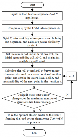
Through comparison, AP algorithm was found to satisfy the above requirements [16, 17]. However, the AP algorithm has difficulty in processing massive data, not to mention converging quickly to the optimal solution. Thus, the core vector machine (CVM) was introduced to improve the AP algorithm [18, 19]. The CVM compresses and processes the original load data, creating a load feature sequence Φ. The workflow of the improved AP algorithm is explained in Figure 5 below.
Figure 5. Flow chart of improved AP algorithm
Here, the improved AP clustering algorithm is adopted to split the data from the 30 appliances into workday sub-sequence and holiday sub-sequence, with the aim to improve the operability of load decomposition and the accuracy of load identification.
As shown in Figure 5, the original sequence was compressed by the CVM into a new sequence Xi:
${{X}_{i}}=\{{{x}_{i}}(0),{{x}_{i}}(1),{{x}_{i}}(2)\cdots ,{{x}_{i}}(l)\}$ (3)
where, l is the length of the sequence; xi(l) is the feature points on the sequence.
Responsibility r and availability a [20] can be respectively computed by:
$r(\beta ,\delta )\text{=}s(\beta ,\delta )-\max \{a(\beta ,j)+s(\beta ,j)\} $ (4)
$a(\beta ,\delta )=\left\{ \begin{matrix} \min \left\{ 0,r(\delta ,\delta )+\sum\limits_{j\ne \beta ,\delta }{\max \left\{ 0,r(j,\delta ) \right\}} \right\} \\ \sum\limits_{j\ne \delta }{\max \{0,r(j,\delta )\}} \\\end{matrix} \right\}$. (5)
where, r(β,δ) is the responsibility of point β relative to point δ; a(β,δ) is the availability of point β relative to point δ.
The household load sequence Φ of N appliances can be described as:
$\Phi =({{Y}_{1}},{{Y}_{2}},{{Y}_{3}},\cdots ,{{Y}_{N}})$ (6)
where, Y1, Y2, Y3, ..., YN are vectors. The load data that correspond to these vectors can be respectively expressed as:
$\begin{align} & {{Y}_{1}}(n)=\{y_{1}^{1}(0),y_{1}^{2}(1),\cdots ,y_{1}^{{{W}_{1}}}(n)\}, \\ & {{Y}_{2}}(n)=\{y_{2}^{1}(0),y_{2}^{2}(1),\cdots ,y_{2}^{{{W}_{2}}}(n)\}, \\ & {{Y}_{3}}(n)=\{y_{3}^{1}(0),y_{3}^{2}(1),\cdots ,y_{3}^{{{W}_{3}}}(n)\}, \\ & \cdots , \\ & {{Y}_{N}}(n)=\{y_{N}^{1}(0),y_{N}^{2}(1),\cdots ,y_{N}^{{{W}_{S}}}(n)\} \\ \end{align}$ (7)
where, YN(n) is load power eigenvectors; yN is power feature point; n is the number of power feature points; N is the total number of loads; WS is the number of all possible working states.
3.3 Load decomposition and optimization
The characteristic load sequence was taken as the known information and matching template, with the hope that the steady-state load features are repeatable and stackable. Repeatability means that the loads can be identified effectively with the same feature index and feature extraction method. Stackability means the characteristic parameters of a single load could be extracted from the overall load data of several operating equipment for state identification. When multiple power loads work at the same time, the total load power always changes with the state of appliances. Therefore, this paper identifies the working state of appliances through load decomposition, and then identify the type of loads. Based on steady-state load features, the local decomposition model can be approximated by [20, 21]:
$\left\{ \begin{align} & {{P}_{L}}(k)=\sum\limits_{i=1}^{N}{\sum\limits_{m=1}^{M(i)}{{{P}_{i.m}}(k)}}+e(k) \\ & {{Q}_{L}}(k)=\sum\limits_{i=1}^{N}{\sum\limits_{m=1}^{M(i)}{{{Q}_{i.m}}(k)}}+e(k) \\ & F(k)={{{P}_{L}}(k)}/{\sqrt{{{P}_{L}}{{(k)}^{2}}+{{Q}_{L}}{{(k)}^{2}}}}\; \\ \end{align} \right.$ (8)
where, PL(k) and QL(k) are the total active power and total reactive power at the k-th sampling point; Pi,m(k) and Qi,m(k) are the active power and reactive power of appliance i at the k-th sampling point in working state m; e(k) is the noise or error at the k-th sampling point.
Among the various types of consumer side loads, some loads have similar features in active power. Sometimes, when the working state of a load changes, it is impossible to obtain the accurate running state vector of the load. Therefore, this paper creates a multivariate identifier based on active power, reactive power, and power factor. For each sampling point, the objective function of optimization can be expressed as:
$\begin{align} & \min F({{P}_{L}}(k),{{Q}_{L}}(k),\Phi ,{{M}_{S}}) \\ & =\left| {{\lambda }_{1}}({{P}_{L}}(k)-{{\Phi }_{P}}({{M}_{S}})) \right| \\ & +\left| (1-{{\lambda }_{1}})({{Q}_{L}}(k)-{{\Phi }_{Q}}({{M}_{S}})) \right| \\ & +\left| {{\lambda }_{2}}({{F}_{L}}(k)-{{\Phi }_{F}}({{M}_{S}})) \right| \\ \end{align}$ (9)
where, $\lambda_{1} \in[0,1], \lambda_{2} \in[0,+\infty)$ are the weight of active and reactive powers and that of power factor, respectively; PL, QL, FL are the real-time measured values of total active power, total reactive power, and power factor, respectively; ΦP, ΦQ, ΦF are the total active power, total reactive power, and power factor of household load sequence Φ found in MS; MS is the sequence of possible working states of all loads, which consists of load states Sh ($h \in[1, N]$):
${{M}_{S}}=\left\{ \begin{matrix} {{S}_{1}} \\ {{S}_{\text{2}}} \\ {{S}_{\text{3}}} \\ \begin{matrix} \vdots \\ {{S}_{N}} \\\end{matrix} \\\end{matrix} \right\}\text{ }{{\text{S}}_{N}}\in {{N}^{*}},{{\text{S}}_{N}}\in [0,{{W}_{S}}]$ (10)
At any sampling point, the working state Sh of a load and its corresponding power are unknown. Based on the characteristic load sequence, this paper attempts to find the optimal power under the working state combination $M_{S}^{\prime}$, which has the smallest Euclidean distance from the currently sampled power, according to the total power of the working states in the state sequence MS. The optimal power is the currently identified power of the target load.
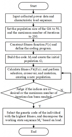
The working states of various loads can be combined in various forms. The heavy computing load drags down the computing speed. To improve the efficiency, the GA was adopted to solve the optimization problem [22, 23]. The workflow of the GA-based solving process is explained in Figure 6 below.
Figure 6. Flow chart of GA-based solving process
4.1 Experimental platform
Our experiments were carried out on the Intelligent Power Management Platform, which has been built on the consumer side of a neighborhood. During the construction of the platform, a smart remote load controller was installed at the door of each resident to detect and control household appliances. The monitoring circuit of the controller is the same as that of the SRLC-based NILM in Figure 4. The power consumption parameters were collected in real time, with the aid of the controller and smart meters. The environmental environment is displayed in Figure 7. The load data of a household were collected by a self-designed software based on Python and MATLAB. With functions like data storage, data processing, and plotting, the software was mainly used to establish, store, and compare the characteristic load power sequence.
Figure 7. Experimental environment
Our experiments involve eight appliances in Table 1, including electric kettle, electric rice cooker, electric oven, hair dryer, microwave oven, TV, LED light, refrigerator, and washing machine. The load data were sampled by the said software at the frequency of 1Hz from 6:30-23:00 during February 9th-23rd, 2020.
4.2 AP clustering and results analysis
The load power data of the household were divided into subsequences based on the usage periods. The data on electric rice cooker, hair dryer, and washing machine were selected for clustering. The clustering results are presented in Table 2. During the calculation, the sum of similarity was used to represent the total distance between each sampling point and its corresponding cluster center [20].
Table 2. The improved AP clustering results of the three appliances
|
Type |
Rice cooker |
Hair drier |
Washing machine |
|
Cluster center /W |
0.00 |
||
|
98.69 |
|||
|
103.17 |
|||
|
0.00 |
125.48 |
||
|
92.03 |
130.49 |
||
|
95.69 |
148.68 |
||
|
0.00 |
230.69 |
167.27 |
|
|
443.38 |
233.07 |
168.89 |
|
|
450.11 |
903.25 |
184.58 |
|
|
452.26 |
912.38 |
201.36 |
|
|
455.56 |
918.58 |
207.34 |
|
|
458.64 |
1206.56 |
221.84 |
|
|
1238.77 |
227.81 |
||
|
1252.43 |
248.39 |
||
|
1266.71 |
261.84 |
||
|
286.33 |
|||
|
320.91 |
|||
|
334.00 |
4.3 Load decomposition and results analysis
During load decomposition tests, the actual line voltage was 230V, and the appliances were connected to the channel of the smart remote load controller via the principle in Figure 4. The decomposition tests were performed on a single load and multiple loads, respectively, with 200 tests for each type of load. Since the characteristic parameters P, Q, and F differ in dimensionality, the normalized root means square error (NRMSE) was employed to measure the load identification accuracy [20, 24]:
$NRMSE=\frac{\sqrt{E({{(\overset{\wedge }{\mathop{\Omega }}\,-\Omega )}^{2}})}}{\max (\Omega )-\min (\Omega )}$ (11)
where, $\overset{\wedge}{\mathop{\Omega}}$ is the total power of the load decomposed by improved AP algorithm; Ω is the total power of the load to be decomposed.
(1) Single-load tests
Single-load tests mainly consider the scenario that only one load is on. To verify our method, the nine loads listed in Table 1 were tested in turn. The serial number of appliances corresponds to the name in Table 1. The identification results of single-load tests are listed in Table 3 below.
Table 3. Identification results of single-load tests
|
No. |
Parameter |
P/W |
Q/Var |
F |
NRMSE/% |
|
21 |
Actual value |
1589.70 |
7.66 |
0.999 |
1.161 |
|
Sample value |
1588.31 |
6.62 |
0.998 |
||
|
4 |
Actual value |
1602.00 |
7.88 |
0.999 |
1.175 |
|
Sample value |
1603.55 |
9.20 |
0.997 |
||
|
17 |
Actual value |
455.00 |
3.07 |
0.999 |
1.199 |
|
Sample value |
457.00 |
3.67 |
0.998 |
||
|
5 |
Actual value |
1205.30 |
27.03 |
0.997 |
1.490 |
|
Sample value |
1206.16 |
28.62 |
0.998 |
||
|
10 |
Actual value |
33.67 |
10.20 |
0.957 |
2.131 |
|
Sample value |
31.02 |
12.77 |
0.925 |
||
|
3 |
Actual value |
105.28 |
25.65 |
0.972 |
2.373 |
|
Sample value |
108.52 |
23.12 |
0.978 |
||
|
19 |
Actual value |
1521.92 |
588.01 |
0.933 |
3.036 |
|
Sample value |
1524.83 |
584.63 |
0.934 |
||
|
16 |
Actual value |
61.94 |
24.29 |
0.931 |
3.020 |
|
Sample value |
64.70 |
22.12 |
0.946 |
||
|
27 |
Actual value |
321.28 |
158.45 |
0.553 |
3.486 |
|
Sample value |
319.44 |
152.79 |
0.575 |
(2) Multi-load tests
Multi-load tests mainly target the scenario that different loads are added in different periods. The nine loads listed in Table 3 were combined into five patterns for the tests. The serial number of appliances corresponds to the name in Table 1. The identification results of single-load tests are listed in Table 4 below.
As shown in Table 2, the identification accuracy was relatively low, when only capacitive or inductive loads were combined. The identification accuracy was slightly better, when capacitive or inductive loads were combined with pure resistive loads, especially if the added load has high power. The identification accuracy was much better, when only resistive loads were combined; in this case, almost all loads were recognized successfully. Low-power loads like LED light were sometimes missed, but eventually fully identified thanks to the optimization ability of the GA. The low missing rate has little impact on actual application.
Table 4. Identification results of multi-load tests
|
No. |
Parameter |
P/W |
Q/Var |
F |
NRMSE/% |
|
4+21 |
Actual value |
3184.51 |
15.28 |
1.000 |
2.097 |
|
Sample value |
3182.35 |
13.89 |
1.000 |
||
|
3+4+ 10+17 |
Actual value |
2191.59 |
41.08 |
1.000 |
2.225 |
|
Sample value |
2194.09 |
43.26 |
1.000 |
||
|
4+16 +17 |
Actual value |
2160.94 |
34.24 |
1.000 |
2.326 |
|
Sample value |
2162.25 |
31.83 |
1.000 |
||
|
16+19 +21+27 |
Actual value |
3480.84 |
780.41 |
0.973 |
3.867 |
|
Sample value |
3484.66 |
776.66 |
0.973 |
||
|
3+10+ 19+27 |
Actual value |
1771.25 |
789.17 |
0.913 |
3.922 |
|
Sample value |
1775.39 |
785.88 |
0.914 |
Based on the principle of NILM and the load parameter detection function of SRLC, the power consumption parameters (e.g. voltage, current, power, and power factor) could be acquired by installing a monitoring device at the supply entrance of power load. There is no need to install sensors within each appliance or load, reducing the investment and maintenance cost of hardware.
The AP algorithm was improved to cluster the collected load data. On this basis, a characteristic load sequence was constructed, which contains multiple steady-state parameters, and used as the reference template for load decomposition and identification. The clustering algorithm is not sensitive to the initial value or outliers, and outputs valid and stable results.
A load decomposition model was built based on the working state and coding information of appliances, and solved by the GA. Our method could correctly recognize more than 96% of loads, especially the loads with the same power or small power. In addition, our method can be easily transplanted onto software platforms, and applied well in various fields.
This work was supported in part by National Natural Science Foundation of China under Grant (No. 61403284), the Young Key Teacher Program of Henan Polytechnic University (No.2019XQG-17), and the Doctoral Scientific Research Foundation of Henan Polytechnic University (No. B2017-20).
[1] Sun, Z.Q., Wang, S.X., Zhou, K., Liu, T.Y. (2016). Automated demand response system in user side based on load disaggregation. Proceedings of the CSU-EPSA, 28(12): 64-69. https://doi.org/10.3969/j.issn.1003-8930.2016.12.011
[2] Chang, H.H. (2012). Non-intrusive demand monitoring and load identification for energy management systems based on transient feature analyses. Energies, 5(12): 4569-4589. https://doi.org/10.3390/en5114569
[3] Chang, H.H., Lin, L.S., Chen, N., Lee, W.J. (2013). Particle-swarm-optimization-based nonintrusive demand monitoring and load identification in smart meters. IEEE Transactions on Industry Applications, 49(5): 2229-2236. https://doi.org/10.1109/IAS.2012.6373990
[4] Suzuki, K., Inagaki, S., Suzuki, T., Nakamura, H., Ito, K. (2008). Nonintrusive appliance load monitoring based on integer programming. 2008 IEEE SICE Annual Conference, Tokyo, Japan, pp. 2742-2747. https://doi.org/10.1109/SICE.2008.4655131
[5] Liang, J., Ng, S.K.K., Kendall, G., Cheng, G.W.M. (2010). Load signature study—Part II: Disaggregation framework, simulation, and applications. IEEE Transactions on Power Delivery, 25(2): 561-569. https://doi.org/10.1109/TPWRD.2009.2033800
[6] Marchiori, A., Hakkarinen, D., Han, Q., Earle, L. (2011). Circuit-level load monitoring for household energy management. IEEE Pervasive Computing, 10(1): 40-48. https://doi.org/10.1109/MPRV.2010.72
[7] Chang, H.H., Chen, K.L., Tsai, Y.P., Lee, W.J. (2012). A new measurement method for power signatures of nonintrusive demand monitoring and load identification. IEEE Transactions on Industry Applications, 48(2): 764-771. https://doi.org/10.1109/TIA.2011.2180497
[8] Gao, Y., Yang, H. (2013). Household load identification based on closeness matching of transient characteristics. Automation of Electric Power Systems, 37(9): 54-59. https://doi.org/10.7500/AEPS201207298
[9] Abdullah-al-nahid, Kong, Y., Hasan, M. (2015). Performance analysis of Canny's edge detection method for modified threshold algorithms. 2015 International Conference on Electrical & Electronic Engineering (ICEEE), Rajshahi, Bangladesh, pp. 93-96. https://doi.org/10.1109/CEEE.2015.7428227
[10] Qi, B., Cheng, Y., Wu, X. (2016). Non-intrusive household appliance load identification method based on fisher supervised discriminant. Power System Technology, 40(8): 2484-2490. https://doi.org/10.13335/j.1000-3673.pst.2016.08.034
[11] Yang, D.S., Kong, L., Hu, B., Yuan, T. (2017). Load identification method based on multi-feature sequence fusion. Automation of Electric Power Systems, 41(22): 72-79. https://doi.org/10.7500/AEPS20170516002
[12] Wang, L.J., Chen, X.M., Wang, G., Hua, D. (2018). Non-intrusive load monitoring algorithm based on features of V–I trajectory. Electric Power Systems Research, 157: 134-144. https://doi.org/10.1016/j.epsr.2017.12.012
[13] Welikala, S., Dinesh, C., Ekanayake, M.P.B., Godaliyadda, R.I., Ekanayake, J. (2019). Incorporating appliance usage patterns for non-intrusive load monitoring and load forecasting. IEEE Transactions on Smart Grid, 10(1): 448-461. https://doi.org/10.1109/TSG.2017.2743760
[14] Chen, S.Y., Gao, F., Liu, T., Zhai, Q.Z., Guan, X.H. (2016). Load disaggregation method based on factorial hidden Markov model and its sensitivity analysis. Automation of Electric Power Systems, 40(21): 128-136. https://doi.org/10.7500/AEPS20160201004
[15] Li, J., Li, W.W., Wang, Z.X. (2013). Research and application of load control based on set point overshoot method. Advanced Materials Research, 805-806: 1022-1026. https://doi.org/10.4028/www.scientific.net/amr.805-806.1022
[16] Frey, B.J., Dueck, D. (2007). Clustering by passing messages between data points. Science, 315(5814): 972-976. https://doi.org/10.1126/science.1136800
[17] Shang, F., Jiao, L.C., Shi, J., Wang, F., Gong, M.G. (2012). Fast affinity propagation clustering: A multilevel approach. Pattern Recognition, 45(1): 474-486. https://doi.org/10.1016/j.patcog.2011.04.032
[18] Tsang, I.W., Kwok, J.T., Cheung, P.M. (2005). Core vector machines: Fast SVM training on very large data sets. Journal of Machine Learning Research, 6(4): 363-392.
[19] Chen, W.L., Cheng, K.M., Chen, K.F. (2018). Derivation and verification of a vector controller for induction machines with consideration of stator and rotor core losses. IET Electric Power Applications, 12(1): 1-11. https://doi.org/10.1049/iet-epa.2016.0654
[20] Xu, Q.S., Lou, O.D, Zheng, A.X., Liu, Y.J. (2018). A non-Intrusive load decomposition method based on affinity propagation and genetic algorithm optimization. Transactions of China Electrotechnical Society, 33(16): 3869-3878. https://doi.org/10.19595/j.cnki.1000-6753.tces.170894
[21] Mengistu, M.A., Girmay, A.A., Camarda, C., Acquaviva, A., Patti, E. (2019). A cloud-based on-line disaggregation algorithm for home appliance loads. IEEE Transactions on Smart Grid, 10(3): 3430-3439. https://doi.org/10.1109/TSG.2018.2826844
[22] Deb, K., Pratap, A., Agarwal, S., Meyarivan, T. (2002). A fast and elitist multiobjective genetic algorithm: NSGA-II. IEEE Transactions on Evolutionary Computation, 6(2): 182-197. https://doi.org/10.1109/4235.996017
[23] Doerr, B., Doerr, C. (2018). Optimal static and self-adjusting parameter choices for the (1+(λ, λ)) genetic algorithm. Algorithmica, 80(5): 1658-1709. https://doi.org/10.1007/s00453-017-0354-9
[24] Egarter, D., Bhuvana, V.P., Elmenreich, W. (2015). PALDi: Online load disaggregation via particle filtering. IEEE Transactions on Instrumentation and Measurement, 64(2): 467-477. https://doi.org/10.1109/TIM.2014.2344373