Alaa Al-Hadidi* | Hamzeh Duwairi
OPEN ACCESS
This paper puts forward a novel model to evaluate the fluid velocity, power and efficiency of a wind turbine under the fluctuating pressure gradient of laminar and turbulent air flows. The operation parameters of a wind turbine were calculated based on the conservation of momentum, under different velocity profiles, fluctuating amplitudes and wave lengths, revealing the effects of fluctuating air pressure gradient on transient power output of the wind turbine. The effectiveness of the proposed model was verified through evaluation of output power, in comparison with a popular statistical tool. The results show that, whether the flow is laminar or turbulent, the pressure gradient has a positive impact on the output power; the enhancement effect is positively correlated with the fluctuation amplitude, and prominent within the early cycles of fluctuations; for turbulent flow, the more intense the flow, the better the output power.
fluctuations, wind turbine, output power, turbulence intensity, Eddy viscosity, boundary layer thickness
Energy is one form of existence and it is the most important component of the universe. Energy could be extracted from both renewable resources and nonrenewable resources [1]. Renewable energy is the type of energy that could harnessed from natural resources while nonrenewable energy (conventional energy) is the energy that formed over time and under several of factors like fossil fuel. All these types of energy require different methods, tools and mechanisms to be extracted and harnessed so as to be beneficial to humanity. Nowadays wind turbines are one of the most promising technology that convert the kinetic energy in the wind to electrical energy. Approximately 2 % of sunlight falling on the surface of the earth converted to wind energy [2]. This is an enormous amount of energy, which surpasses the world's need for consumption in any year. Wind energy has been used in different sectors, most notably: pumping water, electricity production, move ships through pushing their sails, etc.
Kooiman and Tullis [3] studied the effects of unsteady wind conditions on the aerodynamic performance of VAWT. Temporal variation of the wind with respect to the direction and velocity fluctuations was quantified and the corresponding performance of the experimental turbine was compared to the base case wind tunnel performance. Theoretical analysis indicated that the performance of the turbine should depend on wind speed fluctuations, while remaining relatively independent of direction fluctuations. Experimental testing confirmed the independence of the direction fluctuations and quantified the impact of the wind speed fluctuations on the turbine performance. The wind speed fluctuations exhibited minimal impact on the performance when the normalized velocity fluctuations < 15 %, while for greater fluctuations the performance decreased with a roughly linear relationship.
Danao et al. [4] investigated out the effects of steady and unsteady wind on the performance of a wind tunnel scale VAWT. they found that when the VAWT operates in periodically fluctuating wind conditions, overall performance slightly improves if the following are satisfied: the mean tip speed ratio is just above the tip speed ratio of the steady performance, the amplitude of fluctuation is small (<10 %), and the frequency of fluctuation is high (>1 Hz). Within realistic conditions, higher frequencies of fluctuation marginally improve the performance of the VAWT.
Danao et al., [5] investigated the performance of VAWT on a wind tunnel scale with unsteady wind conditions. The wind speed at which testing was conducted was 7 m/s (giving a Reynolds number of around 50,000) with both 7 % and 12 % fluctuations in wind velocity at a frequency of 0.5 Hz. Rotational speed fluctuations in the VAWT were induced by the unsteady wind and these were used to derive instantaneous turbine rotor power. The results showed the unsteady power coefficient (λ) fluctuates following the changes in wind speed. The time average of the unsteady λ with a 7 % fluctuation in wind velocity was very close to that with steady wind conditions while 12 % fluctuations in wind speed resulted in a drop in the mean λ. At mean rotational speeds corresponding to tip speed ratios beyond peak λ, no significant hysteresis was observed for both 7 % and 12 % fluctuations. However, substantial hysteresis is seen for conditions where mean tip speed ratios is below peak λ. Thus, it was found that unsteady free stream causes a drop-in performance of the laboratory scale VAWT tested.
del Campo et al. [6] investigated the aerodynamic behavior of three different vertical-axis wind turbines in wind speeds that vary sinusoidally with time. It was found that the associated power loss becomes significant only when the amplitude of the oscillations in wind speed is high, whereas the frequency of the variation in wind speed is shown to have a minor effect for all practical urban wind conditions.
In this study, a new model has been built to evaluate fluid velocity, power and efficiency of a wind turbine under the effect of the air pressure gradient fluctuations. The performance of a wind turbine under the impact of fluctuating air pressure gradient is being calculated. A study of various operation parameters of a wind turbine is being donated, utilizing conservation principles; continuity and momentum, with wind turbine equations. Different results for velocity profiles, air stream fluctuating amplitude and wave lengths against completely different operation parameters has been determined and plotted, Showing the effects of fluctuating air pressure gradient on transient wind turbine output power. Also, a comparison between the presented model with the available statistical tools methods that usually used to evaluate wind turbine output power has been done.
Air or any other fluid moves according to three fundamental laws and principles of physics: conservation of mass, conservation of energy, and conservation of momentum [7].
Conservation of mass: states that an air mass is neither created nor destroyed. From this principle, it follows that the amount of air mass coming into a wind turbine should equal to that leaving it. In this study, the air was assumed to be incompressible, which mean that the change of air density that occurs as a result of pressure loss and flow is negligible.
Conservation of energy: states that the total energy of an isolated system remains constant, which means that the energy can neither be created nor destroyed; rather, it can only be transformed or transferred from one form to another. This is considered the basis of one of the main expressions of aerodynamics, the Bernoulli equation. Bernoulli's equation in its simple form shows that, for an elemental flow stream, the difference in total pressures between any two points is equal to the pressure loss between these points.
Conservation of momentum is based on Newton's second law; that a body maintains in its state of rest or uniform motion unless compelled by another force that changes its state.
These fundamental principles may be portrayed in terms of mathematical equations; that are expressed, in one form, as unsteady Navier-Stokes equations. Equation (1) indicates that the amount of air mass coming into a wind turbine is equal to that leaving, Equation (2) indicates that the inertia forces is equals to the difference between viscous forces and the integration of the fluctuating pressure gradients of Wind.
incompressible parallel flow, unsteady subjected fluctuation pressure gradients assumption has been made, in order to represent wind velocity and power changes, two flow conditions are considered: one represents laminar flows near cut in velocity and second represents turbulent flows near rated speed velocity.
The dimensionless eddy viscosity (b = 1 + ɛm+) represents laminar flows for b = 1 and turbulent flows for b greater than 1, the value of dimensionless eddy viscosity (ɛm+ = ɛm /ν) are in the range of 0.2 * 105 [8].
$\frac{\partial \mathrm{u}}{\partial \mathrm{x}}+\frac{\partial \mathrm{v}}{\partial \mathrm{y}}=0 \quad \frac{\partial \mathrm{u}}{\partial \mathrm{x}}+\frac{\partial \mathrm{v}}{\partial \mathrm{y}}=0$ (1)
$\frac{\partial \mathrm{u}}{\partial \mathrm{t}}=-\int \frac{1}{\rho} \frac{\partial \mathrm{P}}{\partial \mathrm{x}}+v \frac{\partial}{\partial \mathrm{y}}\left(\mathrm{b} \frac{\partial \mathrm{u}}{\partial \mathrm{y}}\right)$ (2)
The fluctuating pressure gradient is assumed to be:
$-\frac{1}{\rho} \frac{\partial p}{\partial x}=p_{0} \cos (n t)$ (3)
where, Po is the air pressure gradient fluctuation amplitude and n is the number of air pressure gradient fluctuation cycles.
The above equations are a system of second order nonlinear differential equations, which are accompanied by initial and boundary conditions. Here u is the axial velocity, p is the Air pressure, v is the kinematic viscosity which equal to, $\rho$ is the density of air and b indicate the air turbulence level.
The corresponding initial and boundary conditions are:
$\mathrm{u}=u_{\infty}$ at $\mathrm{t}=\mathrm{o}$
$\mathrm{u}=0,$ at $\mathrm{y}=0$ for $\mathrm{t}>0$ (4)
$\mathrm{u}=u_{\infty},$ when $\mathrm{y} \rightarrow \infty$ for $\mathrm{t}>0$
$\hat{\mathrm{u}}$ Variable has been defined as the summation of the velocity and the integration of the fluctuating pressure gradients of the Wind:
$\hat{\mathrm{u}}=\mathrm{u}+\int \frac{1}{\rho} \frac{\partial \mathrm{P}}{\partial \mathrm{x}} d t$ (5)
Substituting Equation (5) into Equation (2), one gets.
$\frac{\partial \hat{\mathrm{u}}}{\partial \mathrm{t}}=v \frac{\partial}{\partial \mathrm{y}}\left(\mathrm{b} \frac{\partial \hat{\mathrm{u}}}{\partial \mathrm{y}}\right)$ (6)
The following non-dimensional variables are adopted to rewrite the governing equation in a proper non-dimensional form:
$u^{*}=\frac{\hat{\mathrm{u}}}{u_{\infty}} \quad \mathrm{y}^{*}=\frac{y u_{\infty}}{v} \quad \mathrm{t}^{*}=\frac{t}{t_{o}}$ (7)
Hence,
$t_{o}=\frac{v}{u_{\infty}^{2}}$ (8)
Substitute above Equations (7-8) in Equations (6) one gets:
$\frac{\partial\left(\mathbf{u}^{*}\right)}{\partial\left(\mathbf{t}^{*}\right)}=\mathbf{b} \frac{\partial^{2}\left(\mathbf{u}^{*}\right)}{\partial\left(\mathbf{y}^{*}\right)^{2}}$ (9)
The following transformation is introduced to reduce the boundary layer equation to an equation with a single independent variable which is, in other words, changing the partial differential equation (PDE) to an ordinary differential equation (ODE):
Let,
$\eta=\frac{A \mathrm{y}^{*}}{t^{*} n} \quad f(\eta)=\mathrm{u}^{*}$ (10)
Hence,
$\frac{\partial(\eta)}{\partial\left({y}^{*}\right)}=\frac{A}{t^{* n}} \quad \frac{\partial(\mathfrak{n})}{\partial\left(\mathfrak{t}^{*}\right)}=-n \mathrm{A} \mathrm{y}^{*} t^{*^{-}(1+n)}$ (11)
Assuming that
$f(\eta)=\mathrm{u}^{*}$ (12)
And hence,
$\frac{\partial\left(\mathbf{u}^{*}\right)}{\partial\left(\mathbf{y}^{*}\right)}=\frac{\partial(f)}{\partial(\mathbf{\eta})} \frac{\partial(\mathbf{\eta})}{\partial\left(\mathbf{y}^{*}\right)}=f^{\prime} \frac{A}{t^{* n}}$
$\frac{\partial^{2}\left(u^{*}\right)}{\partial\left(y^{*}\right)^{2}}=\frac{\partial\left(f^{\prime}\right)}{\partial(\eta)} \frac{\partial(\eta)}{\partial\left(y^{*}\right)}=f^{\prime \prime} \frac{A^{2}}{t^{* 2 n}}$ (13)
$\frac{\partial\left(\mathfrak{u}^{*}\right)}{\partial\left(t^{*}\right)}=\frac{\partial(f)}{\partial(\eta)} \frac{\partial(\eta)}{\partial\left(t^{*}\right)}=f^{\prime} *\left(-n A \mathrm{y}^{*} t^{*^{-}(1+n)}\right)$
Substitute above Equations (13) in Equations (9), the governing equation would be as follows:
$f^{\prime}\left(-n A y^{*} t^{*^{-}(1+n)}\right)=b f^{\prime\prime} \frac{A^{2}}{t^{* 2 n}}$
$-n \frac{\mathrm{n}}{t^{*}} f^{\prime}=\mathrm{b} \frac{\mathrm{A}^{2}}{t^{*^{2 n}}} f^{\prime\prime} \rightarrow 2 n=1 \rightarrow n=\frac{1}{2}$
Then
$f^{\prime \prime}+\frac{n}{2 b A^{2}} f^{\prime}=0$ (14)
To simplify the equation, A is assumed to be $\frac{1}{\sqrt{2}}$, hence the governing equation becomes:
$f^{\prime \prime}+\frac{n}{b} f^{\prime}=0$ (15)
where,
$\eta=\frac{y}{\sqrt{2 v t}}$ (16)
Equation (15) is a linear homogenous second order ordinary differential equation and can be adopted as a replacement to the partial differential Equation (2).
Now the transformed initial and boundary Conditions associated with Equations (4) are:
at $t=0 \rightarrow \eta=\infty$ and $u^{*}=1 \rightarrow f(\infty)=1$
at $\mathrm{y}=0 \rightarrow \eta=0 \quad$ and $\quad u^{*}=0 \rightarrow f(0)=0$ (17)
at $y=y_{\infty} \rightarrow \eta=\infty$ and $u^{*}=1 \rightarrow f(\infty)=1$
Solving equation (15) by adopting the above initial and boundary conditions is outlined below:
Equation (15) can be rewritten as
$\frac{d f^{\prime}}{f^{\prime}}=-\eta \mathrm{d} \eta$
Integrating both sides,
$\ln f^{\prime}=-\frac{\eta^{2}}{2 b}+c_{0}$ or $f^{\prime}=c_{1} e^{-\frac{\eta^{2}}{2 b}}$
Integrating again,
$f=c_{1} \int_{\infty}^{\eta} e^{-\frac{\sigma^{2}}{2 b}} \mathrm{d} \sigma+c_{2}$
The lower limit is arbitrary, and $\infty$ is a good choice.
The boundary condition $f(\infty) \rightarrow 1$ requires that: $c_{2}=1$. The boundary condition $f(0)=0$ requires:
$0=c_{1} \int_{\infty}^{0} e^{-\frac{\sigma^{2}}{2 b}} \mathrm{d} \sigma+1$
$c_{1}=\frac{-1}{\int_{\infty}^{0} e^{-\frac{\sigma^{2}}{2 b}} \mathrm{d} \sigma}=\frac{1}{\int_{0}^{\infty} e^{-\frac{\sigma^{2}}{2 b}} \mathrm{d} \sigma}$
Then $\eta$
$f=\frac{\int_{\infty}^{\mathrm{n}} e^{-\frac{\sigma^{2}}{2 b}} \mathrm{d} \sigma}{\int_{0}^{\infty} e^{-\frac{\sigma^{2}}{2 b}} \mathrm{d} \sigma}+1=1-\frac{\int_{\sigma}^{\infty} e^{-\frac{\sigma^{2}}{2 b}} \mathrm{d} \sigma}{\int_{0}^{\infty} e^{-\frac{\sigma^{2}}{2 b}} \mathrm{d} \sigma}$
Assuming
$z=\frac{\sigma}{\sqrt{2 b}}$
Then
$\mathrm{d} \mathrm{z}=\frac{\mathrm{d} \sigma}{\sqrt{2 b}}$
The new initial and boundary conditions associated with these equations are:
$\begin{aligned} \sigma &=\eta \rightarrow \mathrm{z}=\frac{\mathrm{n}}{\sqrt{2 b}} \\ \sigma &=0 \rightarrow \mathrm{z}=0 \\ \sigma &=\infty \rightarrow \mathrm{z}=\infty \end{aligned}$
Then
$f=1-\frac{\int_{\frac{\pi}{\sqrt{2 b}}}^{\infty} e^{-\frac{(z \sqrt{2 b})^{2}}{2 b} \sqrt{2} \mathrm{d} z}}{\int_{0}^{\infty} e^{-\frac{(z \sqrt{2 b})^{2}}{2 b}} \sqrt{2} \mathrm{d} z}=1-\frac{\int_{\frac{\pi}{2 b}}^{\infty} e^{-z^{2}} \mathrm{d} z}{\int_{0}^{\infty} e^{-z^{2}} \mathrm{d} z}$
But
$\int_{0}^{\infty} e^{-z^{2}} \mathrm{d} \mathrm{z}=\frac{\sqrt{\pi}}{2}$
Then
$f=1-\frac{2}{\sqrt{\pi}} \int_{\frac{n}{\sqrt{2 b}}}^{\infty} e^{-z^{2}} d z$
Hence,
$\operatorname{erfc}\left(\frac{\mathrm{n}}{\sqrt{2 b}}\right)=1-\operatorname{erf}\left(\frac{\eta}{\sqrt{2 b}}\right)=\frac{2}{\sqrt{\pi}} \int_{\frac{\mathrm{n}}{\sqrt{2 b}}}^{\infty} e^{-\mathrm{z}^{2}} \mathrm{d} \mathrm{z}$
Then
$f(\eta)=\operatorname{erf}\left(\frac{\eta}{\sqrt{2 b}}\right)$
And since
$f(\eta)=\mathfrak{u}^{*}$ and $u^{*}=\frac{u+\int \frac{1}{\rho} \frac{\partial P}{\partial x} d t}{u_{\infty}}$
Then
$\mathrm{u}=\operatorname{erf}\left(\frac{\mathrm{n}}{\sqrt{2 b}}\right) *\left(u_{\infty}\right)+\frac{p_{0} \sin (n t)}{n}$ (18)
where,
$\eta=\frac{\mathrm{y}}{\sqrt{2 v t}}$
This equation shows the laminar and turbulent wind speed inside boundary layers, also it shows the effect of oscillating pressure gradient to different wind boundary layers.
The wind power extracted by the rotor blades can be calculated under the effect of the fluctuating pressure gradient by the following equations.
$P(u(0, R))=\frac{1}{2} \rho A u^{3}(0, R) \lambda=\frac{1}{2} \rho \lambda \int_{A 1}^{A 2} u^{3} d A$ (19)
The potential power is calculated by considering the integration on turbine blades center to outside radius where area is (2πrdr) and the radius changes from 0 to R.
$P(u(0, R))=\frac{1}{2} \rho \lambda \int_{0}^{R}\left(\operatorname{erf}\left(\frac{\eta}{\sqrt{2 b}}\right) *\left(u_{\infty}\right)+\frac{p_{0} \sin (n t)}{n}\right)^{3} 2 \pi r d r$ (20)
Rewriting Equation (20) with the dimensionless variable $\eta$, where wind turbine radius (r) plus wind turbine hub height (Hb) is replacing (y) in Equation (18), then:
$\eta=\frac{\left(r+H_{b}\right)}{\sqrt{2 v t}}$ and hence $d \eta=\frac{1}{\sqrt{2 v t}} d r$
Then
$P(u(0, R))=\frac{1}{2} \rho \lambda \int_{\eta_{1}}^{\eta_{2}}\left(e r f\left(\frac{\eta}{\sqrt{2 b}}\right) *\left(u_{\infty}\right)+\frac{p_{0} \sin (n t)}{n}\right)^{3} 2 \pi \sqrt{2 v t}\left(\eta \sqrt{2 v t}-H_{b}\right) d \eta$ (21)
where,
$\eta_{1}=\frac{H_{b}}{\sqrt{2 v t}} \quad \eta_{2} =\frac{r+H_{b}}{\sqrt{2 v t}}$
This power is compared with a power version calculated without the pressure gradient fluctuations effect, on other words, calculating power using Equation (21) with Po=0.
The equation becomes:
$P(u(0, R))=\frac{1}{2} \rho \lambda \int_{\eta_{1}}^{\eta_{2}}\left(e r f\left(\frac{\eta}{\sqrt{2 b}}\right) *\left(u_{\infty}\right)\right)^{3} 2 \pi \sqrt{2 v t}\left(\eta \sqrt{2 v t}-H_{b}\right) d \eta$ (22)
The ratio between the above two versions is an efficient way to study the effect of pressure gradient fluctuations on the output power of wind turbine and is adopted throughout this work.
The results of laminar and turbulent flow under the effect of air pressure gradient fluctuation are presented and discussed, Different figures have been plotted to investigate the effect of the fluctuation of air pressure gradient on a wind turbine using MATLAB software. Also, an actual data from wind turbine data sheet has been used in the model. Table 1 below shows the technical specification for the elected wind turbine (GAMESA G97).
Table 1. GAMESA G97 technical specification [9]
|
Rated power |
2 MW. |
|
Hub height |
78 m. |
|
Diameter |
97 m. |
|
Swept Area |
7390 m2. |
|
Tip speed |
90 m/s. |
To model the laminar flow of air, the variables in equations (21) have been defined as shown in Table 2.
Table 2. Variables definition
|
Variables |
Laminar Flow |
Turbulent Flow |
unit |
|
b |
1 |
15,000 |
Dimensionless |
|
$u_{\infty}$ |
5 |
30 |
m/s |
|
n |
1 |
3 |
cycle/ hour |
|
Po |
0.1 |
4 |
m/s |
|
v |
1.8*10-5 |
1.8*10-5 |
m2/s |
|
$\rho$ |
1.2 |
1.2 |
kg/m3 |
|
$\lambda$ |
0.35 |
0.35 |
Dimensionless |
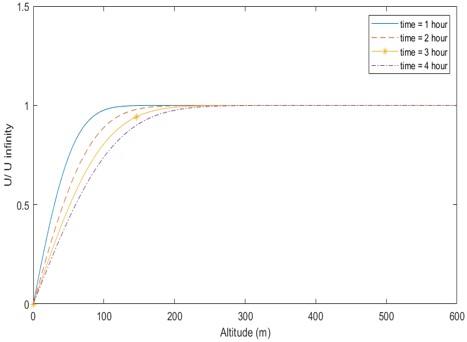
Figure 1. (U/Uinfinity) vs altitude (meter) at different time (laminar flow)
Figure 2. (U/Uinfinity) vs Altitude (meter) at different time (turbulent flow)
Figures 1 and 2 showed the air stream velocity over the maximum air velocity that could be reached in laminar and turbulent flow conditions (U/Uinfinity) for different altitudes and times, it was found that as time is elapsed the boundary layer thickness are increased; this is due to unfavorable friction forces and fluctuating pressure gradients inside boundary layers, it is also clear the small boundary layer thicknesses for laminar flows which equal to around (3) meters. on the other hand, the boundary layer thickness for turbulent flow is higher than it is at laminar flow; this mainly due to the higher shear stress associated with the turbulent flow.
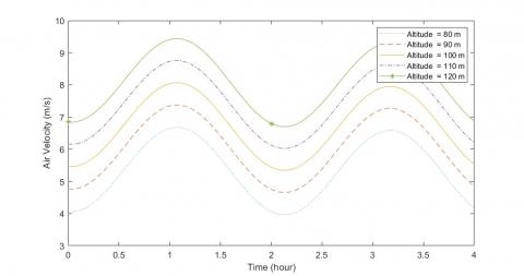
Figure 3 showed the fluctuation in the air stream velocities at different altitude (from 60 meter to 120 meter) for turbulent flow, as shown in the figure increasing altitude lead to an increase in the air stream velocities due to the fact that the boundary layer thickness for turbulent flow is around 300 meter as shown in Figure 2. Also increasing altitudes don’t affect air stream velocities while the flow is laminar since the boundary layer thickness is around 3 meters for laminar flow as shown in Figure (1) which mean that after these three-meter the air stream velocities are recovered thus velocities will be the same.
Figure 3. Air stream velocity (m/s) VS Time (hour) at different altitude (turbulent flow)
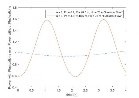
Figure 4. Output power with fluctuation of air pressure gradient over output power without fluctuation of air pressure gradient VS Time (hour)
Figures 4 is used to show the effects the air pressure gradient fluctuation on the wind turbine power output for laminar and turbulent flows, the ratio of the wind turbine power output under pressure gradient fluctuation over the output power without the effect of the air pressure gradient fluctuation has been plotted for a period of 4 hours, the maximum value of this ratio is found to be around 1.03 and the minimum value is around 0.975, with average of 1.0025 while the flow is laminar, and for turbulent flow the maximum value of this ratio is around 1.58 and the minimum value is around 0.588, with average of 1.05 while the flow is turbulent.
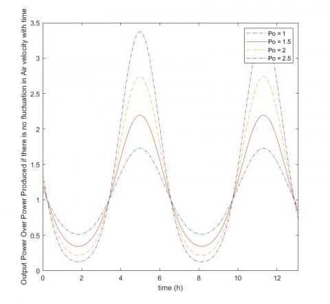
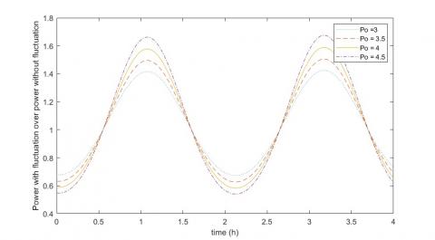
Figure 5. Output power with air pressure gradient fluctuation over output power without air pressure gradient fluctuation VS Time elapse at different (Po) (laminar flow)
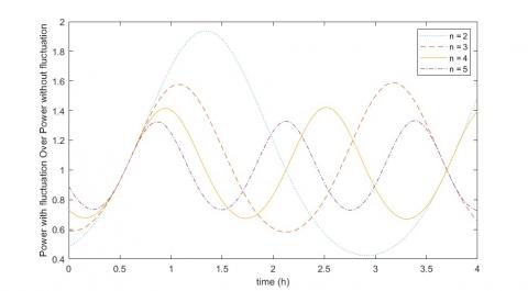
Figure 6. Output power with fluctuation of air pressure gradient over output power without fluctuation of air pressure gradient VS Time at different (n)(laminar flow)
Figures 5, 6, 7 and 8 showed the ratio of the wind turbine power output under the effect of air pressure gradient fluctuation over wind turbine power output without air pressure gradient fluctuation as time is elapsed at different (Po) and (n). As shown in the figures the increasing of (Po) led to an increase of the maximum and minimum values of this ratio. On the other hand, the increasing of frequency (n) led to rapid fluctuation in this ratio, also the maximum value of this ratio at small (n) is higher than it is at large (n).
Figure 7. Output power with air pressure gradient fluctuation over output power without air pressure gradient fluctuation VS Time elapse at different (Po)(turbulent flow)
Figure 8. Output power with air pressure gradient fluctuation over output power without air pressure gradient fluctuation VS Time at different (n) (turbulent flow)
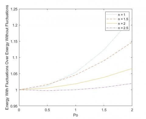
Figure 9. Output energy with air pressure gradient fluctuation over output energy without air pressure gradient fluctuation VS (Po) at different (n)(laminar flow)
Figure 10. Output energy with air pressure gradient fluctuation over output energy without air pressure gradient fluctuation VS (Po) at different (n)(turbulent flow)
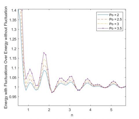
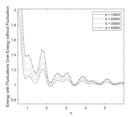
Figure 11. Output energy with air pressure gradient fluctuation over energy output without air pressure gradient fluctuation VS (n) at different (Po)(laminar flow)
Figure 12. Output energy with air pressure gradient fluctuation over output energy without air pressure gradient fluctuation VS (n) at different (Po)(turbulent flow)
To investigate the effect of (Po) on wind turbine energy output, Figures 9 and 10 have been plotted showing the ratio of wind turbine output energy with air pressure gradient fluctuations for a period of (13) hours for laminar flow and for (4) hours for turbulent flow over wind turbine output energy without involving the effect of air pressure gradient fluctuations for the same periods with (Po) at different (n), and it showed that the increasing of (Po) led to an increase in this ratio, which means that increasing (Po) has a positive impact on the wind turbine output power. Also, the figure showed that at low value of (n) the positive effect of increasing (Po) is pronounced compared to the effect at high values of (n) as shown in the Figures and Tables 3 and 4; This is due to the fact that the increasing of frequency (n) reduced the contact time between air streams and wind turbine blades.
Table 3. Output energy with fluctuation over output energy without fluctuation
|
Po n |
0 |
0.5 |
1 |
1.5 |
2 |
|
1 |
1 |
1.012 |
1.05 |
1.12 |
1.22 |
|
1.5 |
1 |
1.016 |
1.046 |
1.09 |
1.15 |
|
2 |
1 |
1.006 |
1.018 |
1.04 |
1.07 |
|
2.5 |
1 |
0.998 |
1 |
1.007 |
1.02 |
Table 4. Output energy with fluctuation over output energy without fluctuation at different (Po) and (n)
|
Po n |
0 |
0.5 |
1 |
1.5 |
2 |
2.5 |
|
2 |
1 |
1 |
1 |
1.007 |
1.015 |
1.025 |
|
3 |
1 |
1 |
1.003 |
1.008 |
1.013 |
1.02 |
|
4 |
1 |
1 |
1.001 |
1.002 |
1.004 |
1.01 |
|
5 |
1 |
1 |
1 |
1.001 |
1.002 |
1 |
Figure 13. Output energy with air pressure gradient fluctuation over output energy without air pressure gradient fluctuation VS (n) at different b
The effects of increasing (n) have been investigated in Figures 11 and 12 showing the ratio of the wind turbine output energy with air pressure gradient fluctuation for a period of (13) hours for laminar flow and for (4) hours for turbulent flow over wind turbine output energy without involving air pressure gradient fluctuation for the same period with (n) at different (Po), It was found that, at small values of (n) the increasing of (Po) led to a decrease in the ratio dramatically however, At higher (n) the ratio became stable and the effect of increasing (n) became negligible as shown in the figures and Tables 3 and 4.
Also, the effects of air turbulence (b) were explored, the ratio of wind turbine output energy with air pressure gradient fluctuation for period of 4 hours over wind turbine output energy without involving air pressure gradient fluctuation for the same period of time has been plotted against both Po and (n) at different air turbulence levels (b). These figures indicate that at all cases as the air turbulence intensity is increased the ratio is increased as shown in the Figures 13 and 14 and the tables 5 and 6 meaning that the increasing of air turbulence level has a positive effect on maximizing the benefits from air pressure gradient fluctuations.
Figure 14. Output energy with air pressure gradient fluctuation over output energy without air pressure gradient fluctuation VS Po at different b
Table 5. Output energy with air pressure gradient fluctuation at different Po and b
|
Po b |
0 |
1 |
2 |
3 |
4 |
|
15000 |
1 |
1.007 |
1.012 |
1.037 |
1.059 |
|
25000 |
1 |
1.011 |
1.029 |
1.055 |
1.089 |
|
35000 |
1 |
1.013 |
1.037 |
1.07 |
1.118 |
|
45000 |
1 |
1.015 |
1.045 |
1.09 |
1.146 |
Table 6. Output energy with air pressure gradient fluctuation at different n and b
|
n b |
0.5 |
1 |
2 |
3 |
4 |
|
15000 |
3.05 |
1.73 |
1.24 |
1.17 |
1.12 |
|
25000 |
4.21 |
2.14 |
1.39 |
1.26 |
1.18 |
|
35000 |
5.36 |
2.55 |
1.54 |
1.34 |
1.24 |
|
45000 |
6.52 |
2.96 |
1.69 |
1.42 |
1.3 |
The results presented in this model have been compared with the results coming from the statistical method of Weibull and Rayleigh which is usually used when calculating wind power.
While Averaging the velocity of wind for a period is not a wise way to determine how much energy could be produced from a wind turbine, since the relationship between the power in the wind and the wind velocity is cubic. For this reason, some statistical tools are implemented like Weibull and Rayleigh statistics method which is normally used in predicting the output energy of a wind turbine considering averaging the value of cubic wind velocity rather than averaging the wind velocity itself [10].
The Weibull distribution is one of the most commonly used lifetime distributions in engineering. It is a useful distribution that can take on the characteristics of any type of distribution, based on the value of the shape parameter k.
Weibull and Rayleigh Statistics is a very general expression that is often used as the starting point for characterizing the statistics of wind speeds which can express mathematically as follows [10]:
$f(v)=\frac{k}{c}\left(\frac{v}{c}\right)^{k-1} \exp \left[-\left(\frac{v}{c}\right)^{k}\right]$ (27)
where, k is called the shape parameter, and c is called the scale parameter.
In fact, when a little detail is known about the wind regime at a site, the usual starting point is to assume k=2. When the shape parameter k is equal to 2, the resulting equation is known as the Rayleigh probability density function:
$f(v)=\frac{\pi v}{2 \bar{v}^{2}} \exp \left[-\frac{\pi}{4}\left(\frac{v}{\overline{v}}\right)^{2}\right]$ (28)
Hence,
$u_{a v g}^{3}=\frac{6}{\pi} \overline{\mathrm{v}}^{3}$ (29)
As shown in Equation (29), Rayleigh statistics method says that the average of the cube of windspeed is 1.91 (6/π) times the average wind speed cubed. Rayleigh statistics enables us to find the average power produced by wind turbine in an acceptable realistic result by the following equation:
$P=\frac{6}{\pi} * \frac{1}{2} * \rho * \pi * R^{2} * \bar{v}^{3} * c p$ (30)
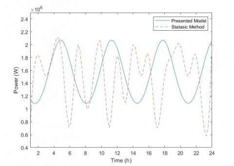
A comparison between the wind turbine output power for one day has been made using the proposed model and using Rayleigh statistics method. The wind speeds used to do the comparison are shown in Table 7.
The wind turbine technical specification shown in Table 8 was then used to calculate the wind turbine output energy for one day using both methods.
In order to model the wind speeds shown in Table 7 in the model presented in this study, MATLAB curve fitting function has been used to calculate Po and n, it was found that (Po) is equal to -0.9858 and (n) is equal to 0.9722.
Then equation (21) has been used to calculate the wind turbine output power for a period of one day
where,
$u^{*}=\operatorname{erf}\left(\frac{\mathrm{\eta}}{\sqrt{2 b}}\right)$ = the ratio of the average wind velocities over $u_{\infty} 0.73$.
$u_{\infty}$=maximum wind speed m/s=13m/s.
Figure 15 showed the expected power output from GAMESA G97 wind turbine using both methods. It was found that the output energy of wind turbine calculated based on the proposed model for one day is equal to (37) MWh, while the energy calculated based on the statistic method for one day is equal to (36.2) MWh, the difference between the two method is slightly low and equal to 2.2 %.
Table 7. Air velocity (m/s) with time (sec)
|
Time (in Hour) |
Wind Speed (m/sec) |
|
1 |
7 |
|
2 |
10 |
|
3 |
9 |
|
4 |
11 |
|
5 |
10 |
|
6 |
7 |
|
7 |
12 |
|
8 |
8 |
|
9 |
9 |
|
10 |
11 |
|
11 |
7 |
|
12 |
10 |
|
13 |
8 |
|
14 |
13 |
|
15 |
9 |
|
16 |
10 |
|
17 |
7 |
|
18 |
9 |
|
19 |
10 |
|
20 |
12 |
|
21 |
9 |
|
22 |
10 |
|
23 |
7 |
|
24 |
12 |
Table 8. GAMESA G97 wind turbine technical specification
|
V (m/s) |
Power (kW) |
λ |
|
3 |
14 |
0.115 |
|
4 |
94 |
0.324 |
|
5 |
236 |
0.417 |
|
6 |
438 |
0.448 |
|
7 |
714 |
0.46 |
|
8 |
1084 |
0.468 |
|
9 |
1508 |
0.457 |
|
10 |
1836 |
0.406 |
|
11 |
1973 |
0.327 |
|
12 |
1992 |
0.255 |
|
13 |
1998 |
0.201 |
|
14 |
2000 |
0.161 |
|
15 |
2000 |
0.131 |
|
16 |
2000 |
0.108 |
|
17 |
2000 |
0.09 |
|
18 |
2000 |
0.076 |
|
19 |
2000 |
0.085 |
|
20 |
2000 |
0.073 |
Table 9. GAMESA G97 wind turbine power and energy output for one day using the statistic method
|
Windspeed (m/s) |
Power (kW) |
Hour/day |
Probability |
Energy (kWh) |
|
7 |
714 |
5 |
0.208333 |
3570 |
|
8 |
1084 |
2 |
0.083333 |
2168 |
|
9 |
1508 |
5 |
0.208333 |
7540 |
|
10 |
1836 |
6 |
0.25 |
11016 |
|
11 |
1973 |
2 |
0.083333 |
3946 |
|
12 |
1992 |
3 |
0.125 |
5976 |
|
13 |
1998 |
1 |
0.041667 |
1998 |
Figure 15. Output power using the statistic method and the presented model in this study verses time
Throughout this study, a model that simulates wind turbine output power under the fluctuating air pressure gradient where the flow is either laminar or turbulent has been built, the model has been solved analytically. After examining the results, one can conclude that:
1- When the flow is either laminar or turbulent the effects of fluctuating pressure gradient is enhancing the wind turbine output power.
2- For turbulent and laminar flow: as the number of air pressure gradient fluctuation cycle is (n) increased, the enhancement resulting from the fluctuation pressure gradient would be minimized till reaching a state that the increase in (n) would insignificantly affects the wind turbine output power. The best performance of wind turbine occurred at low value of (n).
3- For turbulent and laminar flow: as air pressure gradient fluctuation amplitude (Po) is increased, the performance of wind turbine is enhanced.
4- In turbulent Flow: as turbulence intensity is increased the advantage from the fluctuation in air pressure gradient become more apparent.
The following are suggestions for further investigations:
1- Study the effects of laminar and turbulent fluctuating pressure gradient on wind turbine from Blade Theory point of view.
2- Studying the effects of the fluctuating on the structure of wind turbine and its base.
3- Study the effects of laminar and turbulent fluctuating pressure gradient on wind turbine using the experimental methods such like wind tunnel experiment at different conditions and turbulence intensities.
|
A |
Wind Turbine swept area (m2) |
|||
|
b |
Dimensionless Turbulence intensity |
|||
|
E |
Wind turbine output energy (Joule) |
|||
|
Fo |
Fourier Number |
|||
|
Hb |
Wind Turbine hub height |
|||
|
n |
Fluctuation cycle number |
|||
|
p |
Wind turbine output power |
|||
|
Po |
Fluctuation amplitude |
|||
|
r |
Wind Turbine radius |
|||
|
t |
Time |
|||
|
t* |
Dimensionless time variable |
|||
|
u |
Wind velocity |
|||
|
u∞ |
Maximum wind velocity |
|||
|
u* |
Dimensionless Wind velocity variable |
|||
|
$\boldsymbol{\mu}$ |
Dynamic viscosity |
|||
|
v |
Kinematic viscosity |
|||
|
y |
Altitude |
|||
|
y* |
Dimensionless altitude variable |
|||
|
Greek symbols |
|
|||
|
λ |
Coefficient of performance |
|||
|
ɛm ɛm+ $\rho$ $\eta$ $\eta_1$ $\eta_2$ |
Eddy viscosity Dimensionless Eddy viscosity Air density Dimensionless variable Dimensionless variable at hub hight Dimensionless variable at the tip of wind turbine blade |
|||
[1] Praveen, S., Shimi, S.L., Lini, M. (2016). Design and implementation of MPPT technique applied to solar wind hybrid system. International Journal of Advanced Research in Computer and Communication Engineering, 5(7): 604-609. http://doi.org/10.17148/IJARCCE.2016.57120
[2] Tong, W. (2010). Wind Power Generation and Wind Turbine Design an Introduction to Fluid Dynamics. Kollmorgen Corporation, Virginia, USA.
[3] Kooiman, S.J., Tullis, S.W. (2015). Response of a vertical axis wind turbine to time varying wind conditions found within the urban environment. Wind Engineering, 34(4): 389-401. https://doi.org/10.1260/0309-524x.34.4.389
[4] Danao, L.A., Eboibi, O., Howell, R. (2013). An experimental investigation into the influence of unsteady wind on the performance of a vertical axis wind turbine. Applied Energy, 107: 403-411. https://doi.org/10.1016/j.apenergy.2013.02.012
[5] Danao, L.A., Edwards, J., Eboibi, O., Howell, R. (2014). A numerical investigation into the influence of unsteady wind on the performance and aerodynamics of a vertical axis wind turbine. Applied Energy, 116: 111-124. https://doi.org/10.1016/j.apenergy.2013.11.045
[6] del Campo, V., Ragni, D., Micallef, D., Diez, J., Simão Ferreira, C.J. (2015). Estimation of loads on a horizontal axis wind turbine. Wind Energy, 18(11): 1875-1891. https://doi.org/10.1002/we.1794
[7] Tritton, D.J. (1977). Physical fluid Dynamics. Springer Science & Business Media.
[8] Agee, E.M., Brown, D.E., Chen, T.S., Dowell, K.E. (2002). A height-dependent model of eddy viscosity in the planetary boundary layer. Journal of Applied Meteorology, 12: 409-412. https://doi.org/10.1175/1520-0450(1973)012<0409:ahdmoe>2.0.co;2
[9] Siemens Gamesa Renewable. (2015) Power curve. https://en.wind-turbine-models.com/turbines/764-gamesa-g97#powercurve, accessed on 5th February 2019.
[10] Masters, G.M. (2004). Renewable and Efficient Electric Power Systems. John Wiley & Sons.