Ahmed N.E.I. Ayad* | Wafa Krika | Houari Boudjella | Farid Benhamida | Abdessamad Horch
OPEN ACCESS
The purpose of this study is to evaluate the electromagnetic emission of the overhead power line, because these power line generate electromagnetic interaction with other objects near to it. The novelty of this work shows a numerical simulation of the electromagnetic field of the 400 kV line in both permanent and transient states at different positions, based on the finite element method using numerical software. Through the results of this study, it was found that the electromagnetic field in the transient state is very important. The findings of this research can be used to evaluate the field created around transmission lines in order to determine their impact on the environment and human health.
electromagnetic pollution, power line, transient, finite element method, emission
The development and extension of very high voltage electrical networks (VHV) generate and multiply the interactions and electromagnetic problems [1-2] which have a negative effect on environmental risk and human health, moreover they could expose the peoples working around them to serious diseases [3-5].
There are several experimental and simulation studies on electromagnetic characteristics near the power line [5-6]. The most of works is based on the evaluation of the product field around and near the power lines and comparing it with international norms [2-4], other studies have been carried out on the influence of the intensity of the electromagnetic field on the health and the environment [3-4], there are even studies on the reduction of the intensity of the field under the electric lines thanks to technical solutions [7-8]. But all these works have been studied in the steady state; the novelty of this paper is the application in a transient state with presence of defects in the electrical network. Our aim is the simulation of the electromagnetic field in the presence of the various defects in order to have results throws a new light on the electromagnetic pollution in the transient case.
A very good modeling of the electromagnetic characteristics of the electric lines depends to several parameters such as: the characteristics of the electric cables (conductivity, wire shape, cross-section, etc.), the height of the lines, the geometric and structural characteristics of the pylons, the frequency disturbing signals, and the distance between the conductors and the environment characteristics (air, water, etc.) [6-7].
In this paper, we use the electrostatic and magnetostatic modules of the COMSOL Multiphysics software for the simulation to evaluate the electromagnetic pollution of the VHV electric transmission lines. Our work aims to simulate and show the radiated emission of the electromagnetic field produced in the vicinity and around a high voltage electric line by the finite element method. Furthermore and in order to see the variation of the intensity of the field in both permanent and transient cases in different positions, a new simulation of the electromagnetic field under a short circuit and overvoltage faults is proposed.
Each phase is consisted of a horizontal bundle of two conductors of 61 wire separated by 45 cm. The total section of a sub-conductor equals 590 mm2. Figure 1 shows the model of a very high voltage electric line of 400 kV. Its characteristics are listed in Table 1.
Figure 1. Geometry of the VHV electric transmission line
Table 1. Characteristics of the very high voltage line [11]
|
The distance between the phases and the ground (m) |
30 |
|
Conductor diameter (m) |
31.5∙10-3 |
|
The distance between the phases (m) |
16.2 |
|
Voltage (kV) |
400 |
|
Current (A) |
2500 |
The most of electromagnetic phenomena are governed by Maxwell's partial differential equations, which must be adapted to the medium to several domains of the studied device. Thus, due to the slow variations of electromagnetic fields in low frequency (vary slowly over time), Maxwell's equations are converted into electrostatic and magnetostatic equations for the static regime [9-11]. We start with the following system of equations:
$\left\{ \begin{align} & \text{rot}\mathbf{H}=\mathbf{{J}'} \\ & \mathbf{D}=\varepsilon \mathbf{E} \\ & \mathbf{{J}'}=(\sigma +\text{j}\omega \varepsilon )\mathbf{E} \\ & \mathbf{B}=\text{rot}(\mathbf{A}) \\\end{align} \right.$ (1)
With E: electric field, H: magnetic field, A: magnetic vector potential, J: the current density, B: magnetic flux density, D: electric induction.
By applying the law of Gauss and the law of Maxwell Ampere, we will have the equation (2):
$\text{rot}\mathbf{H}=\text{rot}({{\mu }^{-1}}\mathbf{B})$ (2)
We substitute the expression of magnetic flux density B in Maxwell-Faraday equation of electromagnetic induction ($rotE=-jωB$), we obtain:
$\text{rot}\mathbf{E}=-\text{j}\omega (\text{rot}\mathbf{A})=\text{rot}(-\text{j}\omega \mathbf{A})$ (3)
The combination of the preceding equations gives:
$\text{rot}({{\mu }^{-1}}\text{rot}\mathbf{A})=(\sigma +\text{j}\omega \varepsilon )\left( -\text{j}\omega \mathbf{A} \right)$ (4)
After substitution, we obtain the formula of the final partial differential equation for the inductive effect for the following variable magnetic vector potential A in magnetostatic:
$-\omega {}^\text{2}\varepsilon \mathbf{A}+\text{j}\omega \sigma \mathbf{A}+\text{rot}({{\mu }^{-1}}\text{rot}\mathbf{A})=0$ (5)
The interface of Magnetic Fields in the software uses equation (5) to determine the value of magnetic vector potential A, and consequently, the values of all fields derived from it (the magnetic field H and the magnetic flux density B). The electric current of the three phases is as follows [11-12, 14]:
${{I}_{a}}={{I}_{0}}\ ,\ \ {{I}_{b}}\ \ ={{I}_{0}}{{e}^{-\text{j}\frac{2\pi }{3}}}\ ,\ \ \ {{I}_{C}}\ \ ={{I}_{0}}{{e}^{\text{j}\frac{2\pi }{3}}}$ (6)
The resolution of the model in 2D by the law of the current conservation in the electrostatic frequency domain is realized by the following equations:
$\left\{ \begin{align} & \mathbf{E}=-\text{grad}\mathbf{V} \\ & \text{div}\mathbf{D}=\rho \\ & \text{div}\mathbf{J}=-\text{j}\omega \rho \\\end{align} \right.$ (7)
When Faraday’s law evaluates to zero in static case, we have:
$\text{rot}(\mathbf{E})=-\text{j}\omega \mathbf{B}=0$ (8)
The including of the displacement current in the current definition gives: $divJ'=0$ and $J'=σE+jωD$ for the current conservation law and the current definition, respectively we will obtain the following partial differential equation (9) for the variable V:
$-\text{div}((\sigma +\text{j}\omega \varepsilon )\nabla V)=0$ (9)
The interface of the "Electric Currents" uses this conservation law to determine the value of V in the domains. For the limits of this model, several Dirichlet conditions are used. The electric voltage of the three phases is as follows [12, 14, 15]:
${{V}_{a}}={{V}_{0}}\ ,\ \ {{V}_{b}}\ \ ={{V}_{0}}{{e}^{-\text{j}\frac{2\pi }{3}}}\ ,\ \ \ {{V}_{C}}\ \ ={{V}_{0}}{{e}^{\text{j}\frac{2\pi }{3}}}$ (10)
We will use the magnetostatic module for the modeling and calculation of the magnetic field produced near to the electric transmission lines [12, 16].
(a) The distribution of the magnetic field around of transmission line
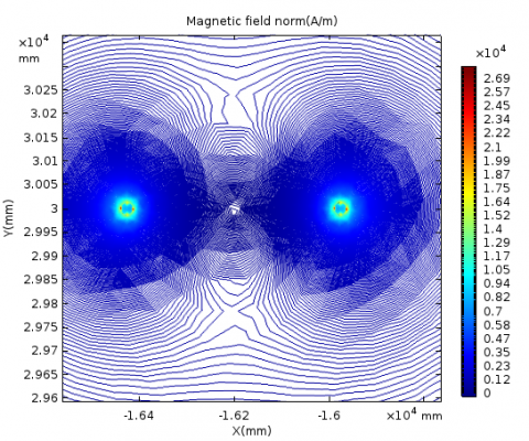
(b) Magnetic field concentration in single phase
Figure 2. The distribution of the magnetic field
Figure 2 shows the radiation emission of magnetic field lines (norm is the magnitude of the variable or absolute value of the magnetic field) in the vicinity as well as under the VHV electric line. The distribution of the field is very important in the very high voltage lines because of the great intensity of the current in the three cables of each line. There are always electromagnetic interference (EMI) between the electric lines as the both inductive and capacitive phenomena between the phases and ground.
5.1 Calculation of the magnetic field near the overhead transmission line
The simulation result shows the horizontal and vertical distribution (along the two axes x and y) of the multi-level magnetic field below the overhead electrics lines (with Hmax=380 A/m). Figure 3 shows the shape of the magnetic field as a function of the distances at several levels with respect to the ground. Moving away from the electric cables, the magnetic field decrease and will be less important in both directions.
Figure 3. Measurement of the magnetic field near the VHV line
5.2 The presence of a short circuit fault in an electrical phase
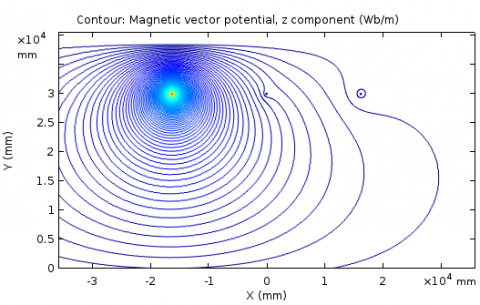
Short circuit current: the circulation of a short circuit current (ICC=45 kA) in an electrical phase gives a large magnetic field. Figure 4 shows an intense and very important magnetic field, unlike the other two phases not affected by the short circuit because of the power transmitted during the short-circuit phase. The maximum amplitude of the magnetic field with short circuit is eighteen times the nominal value (7000 A/m see Figure 5) [12-14].
Figure 4. Magnetic vector potential with a short circuit fault in single phase
Figure 5. Measurement of the magnetic field with a short circuit in a phase
5.3 The calculation of the electric field near the VHV line
The representation of the electric field requires the use of the electrostatic module.
Figure 6. Electric field near overhead transmission line
Figure 6 shows the calculation of the electric field at several levels, it increases and reaches the maximum near the three electric cables, even near and below the line.
When moving away from the x-axis with a distance x=± 100 m, the values of the electric field will be low. So it starts to decrease according to the distance.
5.4 The presence of an overvoltage fault
The circulation of an overvoltage (U=680 Kv between a single phase to ground) in electric phase gives rise to an important electric field [13-14]. The distribution of the electric field is very strong next and close to phases affected by the overvoltage fault (the maximum amplitude is 100 kv/m) see Figure 7.
In abnormal operating conditions the electromagnetic field under very high voltage overhead line is proportionally with the level of current and voltage. The field at other voltages or currents is proportional to the reference case of steady state (the magnetic field increases eighteen times the nominal value of current and the electric field increases three times the nominal value of voltage).
Figure 7. Calculation of the electric field near overhead transmission line with overvoltage
Table 2. The electromagnetic field at 1.7m and 29 m under power transmission lines
|
|
Electric Field Kv/m |
Magnetic Field μT |
||||
|
Distance y(m) |
Limit |
State |
Fault |
Limit |
State |
Fault |
|
1.7 |
5 |
2 |
5.3 |
100 |
9 |
235 |
|
29 |
10 |
40 |
105 |
500 |
516 |
900 |
Table 2 summarizes the comparing of the simulation results with recommendation of the European Commission (EC/519/1999 for public, and EC/402004 for workers) concerning the limits of exposing to low frequency electromagnetic fields, for our study: 1.7 m and 29 m height above the ground.
The presence of electricians under the line of a length y=1.7 m exposes them to an electromagnetic field below normal standards and above standards in case of defects. When the electricians are near to an electric cables at a vertical distance y=29 m), they are exposed to very important values of the electromagnetic field in normal and above all abnormal cases. (The magnetic field is twice as high of the limit in case of short circuit and ten times the value of the electric field in overvoltage).
Through a numerical simulation by finite element method using the COMSOL Multiphysics software, the present paper studied the distribution of the electromagnetic field of the overhead electrical transmission line of 400 kv, for frequency of 50 hertz with neglecting the effect of the ground wires. The finite element method is fast, reliable and accurate; it can analyze any structure with complex geometry and non-linear characteristics.
Based on the results obtained, it can be drawn that the circulation of a short circuit current of 45 kA in electrical phase gives an intense magnetic field (of 7000 A/m) because of the important power transmitted during the short-circuit phase. In the other hand, the presence of an overvoltage fault of 680kv between phase and ground gives an important and strong distribution of electric field (100 kv/m). It can be concluded that the electromagnetic field at several levels increases near and under the line mostly in transient state, so it varies inversely with the distance.
The comparison of the results chows that the electromagnetic field is higher than the limits required by recommendation of the European Commission in the case of the presence of defects. For the perspectives, our objective is to study the electromagnetic aggressions of transmission line and found new technical solutions to minimize the interferences and improved the level the electromagnetic compatibility devices.
[1] Cigre A. (1980). Electrical and magnetic fields generated by transmission networks, example of calculation of electromagnetic disturbances by the CIGRE method. International Conference of Large High-voltage Electrical Networks, Paris Edition Dunod, pp. 21-43.
[2] Kulkarni G, Gandhare WZ. (2012). Proximity effects of high voltage transmission lines on humans. Int. J. on Electrical and Power Engineering 3(1): 1-11. https://doi.org/01.IJEPE.03.01.11
[3] Dib D, Mordjaoui M. (2014). Study of the influence high-voltage power lines on environment and human health (case study: The electromagnetic pollution in Tebessa city, Algeria). Journal of Electrical and Electronic Engineering 2(1): 1-8. https://doi.org/10.11648/j.jeee.20140201.11
[4] Tourab W, Babouri A, Nemamcha M. (2011). Characterization of the electromagnetic Environment at the vicinity of power lines. 21st International Conference Exhibition on Electricity Distribution, CIRED11, pp. 16-21.
[5] Tourab W, Babouri A. (2016). Measurement and modeling of personal exposure to the electric and magnetic fields in the vicinity of high voltage power lines. Safety and Health at Work 7(10): 102-110. https://doi.org/10.1016/j.shaw.2015.11.006
[6] Guo Y, Wang T, Li D, Yang H, Huang H. (2010). The review of electromagnetic pollution in high voltage power systems. Proceedings - 2010 3rd International Conference on Biomedical Engineering and Informatics (IEEE BMEI 2010), pp. 1322-1326. https://doi.org/10.1109/BMEI.2010.5639262
[7] Rachedi BA, Babouri A, Berrouk F. (2014). A study of electromagnetic field generated by high voltage lines using COMSOL multiphysics. Institute of Electrical and Electronics Engineers IEEE 1(2): 2-14. https://doi.org/10.1109/CISTEM.2014.7076989
[8] Djekidel R, Mahi D, Ameur A, Ouchar A, Hadjadj M. (2013). Calcul et atténuation du champ magnétique d’une ligne aérienne HT au moyen d’une boucle passive. Mediamira Science Publisher 54(2): 103-108.
[9] Ahmadi H, Mohseni S, Shayegani A. (2010). Electromagnetic fields near transmission lines problems and solutions. Journal of Environ Health. Sci. Eng 7(2): 181-188. https://doi.org/10.1186/1735-2746-181-188
[10] Bhanuprasad N, Umesh KS. (2018). Location and detection of downed power line fault not touching the ground. European Journal of Electrical Engineering 20(3): 347-362. https://doi.org/10.3166/ejee.20.347-362
[11] Rachidi F. (1993). Formulation of the field to transmission line coupling equations in terms of magnetic excitation field. IEEE Transactions on Electromagnetic Compatibility 35(3): 404-407. https://doi.org/10.1109/15.277316
[12] Smahi W, Slimani A. (2018). Simulation of a radiated aggression of an electric cable. Ph.D. Department of Electrical Engineering, Kasdi Merbah University.
[13] Meunier G. (2013), The Finite Element Method: Theory, Implementation, and Applications’ Book 2013, 395 hardcover Wiley.
[14] Theory for the Magnetic Fields. (2012). No Currents Interface User´s Guide magnetostatic equation AC/DC Module May Multiphysics software COMSOL 4.32012 www.comsol.com/support /releasenotes/4.2/acdc
[15] Bellaredj A. (2016). Design and simulation of a 220KV electric transmission overhead line. Ph.D. Department of Electrical Engineering, Aboubakr Belkaid University.
[16] Yalaoui N. (2017). Calculation of the linear impedance matrix of the line-cable system with the finite element method. Ph.D. Department of Electrical Engineering, Montréal University Canada.