Olatunbosun O. Kafisanwo* | James S. Abe | Ayodele O. Falade
OPEN ACCESS
Traditionally, sonic and density logs are vital components during the generation of synthetic seismogram. However, sonic logs as observed in many studies, often have poor quality or even absent in some cases. This work is a case study for the transformation of resistivity logs to pseudo sonic logs for the generation of pseudo synthetic seismogram considering the effect of gas. This research studies the relationship between resistivity and sonic logs in order to utilize the former for the generation of pseudo synthetics when sonic log is absent or poor. Standard synthetic seismograms were first created conventionally using sonic and density logs as inputs. The sonic log values were then plotted against the corresponding resistivity values for each well to derive their relationship using both linear and polynomial functions. Generally, the crossplot shows a fair correlation but some scattered plots were observed. Further probe into these observed anomalies revealed the areas to be gas saturated. A better correlation was achieved within affected zones by doing independent crossplots for previously gas delineated units. The standard synthetic generated were used as control for the pseudo synthetics and better correlation is observed when compared with the previous pseudo synthetics that does not acknowledge gas-effect.
resistivity, crossplot, transforms, geology, seismogram, pseudo-synthetic, petrophysics, gas, linear
A synthetic seismogram is a direct one-dimensional model of the acoustic energy travelling through inhomogeneous layers of the earth [1]. They are generated by convolving the reflectivity series, derived from digitized sonic and density logs, with seismic extracted zero phased wavelet.
The importance of a quality synthetic seismogram and good seismic-to-well tie in seismic interpretation cannot be over-emphasized, as this determines the event (i.e. peak, trough or cross-over) that will be picked as horizons across seismic lines. Moreover, well logs are point data with higher vertical resolution (at a particular point) than seismic data whose strength lies in its horizontal resolution [2]. Therefore, it is vital to produce a reliable synthetic seismogram that can be used as a control to check the quality of seismic data at well points during seismic-well tie process. Picking the wrong event on a seismic line can be misleading and detrimental as far as seismic interpretation is concerned. In fact, this might eventually lead to drilling of dry holes which cost fortune.
Sonic logs which measures the continuous interval transit time of formations with respect to depth has various applications during well log interpretation. One major use of this log is its input along with density log in the generation of synthetic seismogram.
However, sonic log has been observed to be absent or poor in some dataset. This deficiency might be as a result of hole rigorosity (i.e. when acoustic logs are not corrected for the effect of wellbore irregularities encountered during logging). According to Halderson and Dasleth [3], it could lead to erratic readings in concerned areas. Another factor that might affect the quality of sonic logs is cycle skipping (common in thick shale). This is the incidental delay in interval transit time signal, with resulting increase in amplitude signal that does not represent the true value when it eventually arrives.
We carried out some literature review on some of the methodologies used in previous studies pertaining to this topic. Most of these methods does not put consideration the influence of hydrocarbon, especially gas in reservoir units.
Many researchers including Acvedo and Pennington [4], Faust [5] and Quadir et al. [6] carried out transformation of different log types to pseudo-sonic logs. At first, their work was informed by the observed similarity in signature of the logs with sonic log. This means that the curves do not necessarily have the same unit of measurement, amplitude among other disparities that might exist between them. Quadir et al. [6] tried to create pseudo synthetic seismogram using gamma ray logs in highly radioactive sands. Kung et al. [7] also proposed a technique which basically involves conversion of neutron logs to pseudo sonic logs for the generation of synthetic seismogram in gas saturated clastic rocks. Although there exist some limitations, their results reveal that their objective is empirically and better results can be achieved by treating gas saturated zones in isolation.
Conversely, Dos Santos et al. [8], Lee [9], Faust [10] do not consider the effect of gas formation. This makes their approaches vulnerable in gas formations and even in areas occupied with salty connate water. Also, Kim [11] did not examine the effect of gas and dissolved salt present in connate water. He utilized a method that involves applying a higher order polynomial function on the crossplots with the whole formation captured by the well logs to extract the equations used for the pseudo sonic transformation, not considering the constituents of the formation. Granted, some of these approaches have contributed their own quota to the oil and gas industry for years. Regardless, the pitfalls which is their application in gas formations cannot be disregarded.
Faust [5] proposed a transform which involves using resistivity log values to estimate compressional sonic based on the signatures of resistivity and p-wave sonic. However, he found out that this transform would not work in gas bearing reservoirs, which is known to have a low density. He further posited that, unless the resistivity log utilized is one recorded under a condition where the invaded zone was properly flushed with mud filtrate, the result of the pseudo sonic transform will not fairly match the real sonic log and the corresponding pseudo synthetic log generated with it will not be in sync with the standard synthetic. Therefore, it is necessary to have enough information about the type of resistivity log to be utilized, especially the conditions under which such is logged and recorded.
Alberty [12] utilized Gassmann’s equation to study the effect of hydrocarbon on sonic values. His result shows that hydrocarbon, especially gas, has a non-linear effect on sonic values. Kung et al. [13] considered the effect of gas by using a methodology that involves creating independent crossplots for different geological units in the Fanpokeng gas field of northwestern Taiwan. Although, their method aided a better correlation in different formations when compared to previous approaches that focused on the entire formation. However, it does not directly address the irregularities experienced in gas saturated zones. Therefore, there is need to further delineate these zones and focus on them to correct for observed anomalies. This work intends to directly address the presence of gas in a formation, as a major factor that affects the transformation of resistivity logs to pseudo sonic logs by treating them independently.
2.1 Basic principles
Indeed, well logs are known to be ground truth with higher vertical resolution than seismic. However, this might not be completely true in some instances, as some errors might occur during the logging process. Inhomogeneous petrophysical properties (e.g. differences in fluid content, lithology, compaction, etc.), borehole environmental conditions and logging parameters (e.g. logging speed, signal generation and detection) might affect the quality of logs.
Despite being less sensitive to borehole conditions, sonic logs can also be erroneous. Under normal circumstances, sonic log signals decrease with increase in p-wave velocity and increasing depth of burial [14]. Misfit in signals may occur as a result of noise commonly incorporated in log signal and as a result of utilizing disparate frequencies. For this reason, acoustic logs are normally corrected with checkshot data. Moreover, Omuvwie and Tummala [15], in their study of the impact of borehole irregularities on acoustic logs, discovered that washouts affect sonic and density logs more significantly than commonly acknowledged, and the quality of sonic log has a substantial impact on the quality of subsequent synthetic seismogram and inversion used in reservoir characterization. This is one of the bases for the search of an alternative log with less effects.
Similarly, density logs are also greatly influenced by borehole conditions like washouts. These borehole conditions might not really affect the use of the log for measurement of porosity. However, the values gotten from such logging environment will eventually contribute to the quality of generated synthetic seismogram. Because of these irregularities, it is advised that corrections should always be done during and after acquisition in order to ascertain the quality of the log. It is recommended to always run a caliper log to compliment density log interpretation. Also, Asquith [16] in his study proposed that any density value whose correction exceeds 0.20g/cc should be tagged as invalid.
Anderson and Newrick [17] suggested that the easiest way of identifying the effects of these borehole condition is by considering it with caliper logs in order to have an idea of what the hole condition looks like in the zones. In summary, they suggested that other log types available for a well should be considered to complement the information on density logs. This will help to reconstruct a better replacement for affected intervals. The quality of a synthetic does not only depend on density and sonic logs. It also depends on the quality of the other available well logs types, the ability to extract a representative wavelet from seismic, among other factors.
Apart from the quality of logs and extracted seismic wavelet, other possible factors that can influence the output of a synthetic seismogram (i.e. in terms of time/depth shift, polarity and frequency) include the workflow and software used for its generation [17].
Generally, the typical display of resistivity log and sonic log curve are analogous. The visually observed similarities between these two signals is one of the bases for the attempt to closely study and generate a relationship between them.
Prior to the transformation, the correlation between these two similar curve types were scrutinized putting various factors into consideration (i.e. porosity, compaction, temperature, pressure, presence of shale, gas effect, salinity, etc.) that can influence the data in some formation.
Firstly, compaction as one of the factors considered, can affect the values of both resistivity and sonic logs. Under normal circumstances, with no overpressure zone encountered, compaction is expected to increase with increasing depth and so also is resistivity. On the other hand, sonic ITT (Interval Transit Time) values decreases with increasing compaction. This response causes both logs to cross each other when viewed on the same track (the scale of sonic log is reversed and increases from left to right while resistivity log increases from right to left).
Secondly, porosity as one of the factors that might affect the responses of the logs, can be derived from sonic log as an acoustic log and in some cases with resistivity log. Both logs show similar signature when passing via a brine saturated permeable formation [16]. However, the presence of gas in this type of formation will cause the curve to deflect from the norm.
The presence of mud also influences the output of sonic interval transit time values. Under normal circumstances, the first arrival of P-wave should be one that has travelled through the target formation. However, in some instances when the Tx-Rx is smaller than the critical distance, in a typical large diameter hole, the P-wave signal that has travelled through the mud arrives first leading to a chaotic log response. Another analogous problem that arises as a result of mud invasion is Altered Zone Arrival. This is a situation in which the void between the real formation and the borehole wall is filled with material such as solid mud with higher pressure in overbalanced drilling or even fractured materials with lower pressure mud in pressure depleted reservoir. This pressure difference between the infill material and the real formation affects the travel of acoustic waves and the corresponding sonic log response.
Figure 1. Generation of synthetic seismogram
Likewise, since resistivity distribution in any formation is a function of both rock components and fluid characteristics, the infiltration of drilling mud will impact on the measurement of this physical property in concerned areas. Formation mud invasion is possible during drilling because the pressure of the mud has to be kept slightly higher than that of the formation in order to carry out its functions effectively and prevent terrible drilling event like blow-outs. This difference in pressure aids the infiltration of drilling mud into porous and permeable rock units. Akinsete and Adekoya [18] tried to study the effect of mud filtrate invasion on well log measurements. Concerning resistivity, they concluded that, although both medium and induction logs can be largely affected by invading filtrates (depending on the radial distance of invasion from the wellbore, formation fluid and mudcake properties), measures such as judicious Mud Conditioning, Logging While Drilling (LWD) and curve correction can significantly reduce the errors garnered during well log acquisition.
Again, the property of rock units embedded in a formation is also one of the factors that influence the output of well log signals and resistivity log is not an exception. Therefore, their physical characteristics such as mineral constituents, volume of pores and their connectivity should be put into consideration in order to get a log that reflect the formation properties as accurate as possible. However, unlike other field with complex mineralogy, this is not a problem in the Niger Delta which is the study area because it consists of majorly sands and shales.
The basis of synthetic seismogram is the Zoeppritz’s equation, which is calculated as the product of velocity and density of subsurface layers. The generation of a synthetic seismogram requires velocity and density. The inverse of sonic log is used to replace velocity data which might be absent when calculating acoustic impedance because of the observed inverse relationship between the two logs. The acoustic impedance within each acoustic layer is used as input in the reflectivity series formula which is then convolved with a zero phased seismic wavelet to create a synthetic seismogram. Figure 1 shows an example of the process of generating a typical synthetic seismogram. Eqns. (1), (2), (3) and (4) below shows the mathematical representation of this process.
Zn= $\rho$nVn (1)
Vn= 1/$\Delta$Tn (2)
Zn= $\rho$n /$\Delta$Tn (3)
Rn= (Zn+1+Zn)/ (Zn+1-Zn) (4)
Zn = acoustic impedance of layer n
$\rho$n = density of reflective surface n
Vn = velocity of reflective surface n
$\Delta$Tn = sonic interval transit time of surface n
Rn = reflective index of layer n.
Faust [5] empirically study the relationship between velocity and resistivity. He observed that, while velocity depends on the elasticity of a material, resistivity deals with the electrical charge transport capability. Therefore, the relationship was most likely due to the dependence of both properties on porosity. Porosity is the percentage of pore space in a rock and it can be measured using three types of well logs which include density log, sonic log and neutron log.
Satoshi and Koji [19] attempted to study the relationship between porosity and velocity. The crossplot of the properties shows that velocity generally increases with decrease in porosity. However, the data was found to be dispersed in some areas. Their study further reveals that these irregularities were as a result of clay minerals in the pore spaces. Nabway and Kassab [20] also found out that the amount of clay and the manner of distribution are important factors that contribute to change in porosity.
Another factor that influence the values of these logs is the presence of shale in the formation. Resistivity is low in shale because it contains high bound water. However, sonic values increase in shale formations. Therefore, the two logs will deflect to the left in this scenario.
Hacikoylu et al. [21] studied Faust’s equation and they proposed that the method can only be applied in consolidated sandstones with low clay content and porosity within the range of 5% to 20%. Therefore, it should not be applied in shales or unconsolidated materials.
Apart from compaction, porosity and the presence of shale. Another factor that can alter these logs is the presence of dissolved salt in formation water. Dissolved salt in formation water results in high conductivity with corresponding low resistivity values that increases with increasing depth. On the other hand, sonic values will increase in this kind of environment because of the presence of the dense salt. The response here is such that both curves deflects leftwards.
Concerning gas effect, Alberty [12] and many other researches have studied the response of sonic in gas formation using sonic logs that have being corrected for hole rigidity. They found out that sonic log values have a sharp and non-linear increase when it gets into gas zones and then becomes more constant as it exits gas formation. Resistivity logs also show abrupt increase in values as it gets into gas zones. However, it shows a linear trend unlike sonic logs. This relationship calls for a better study in order to get a better understanding of such irregular zones.
The impact of water and oil is another affect that should be considered, since oil possesses a lower conductivity than formation water which are salty and highly conductive, the resistivity log response in formations with presence of these two liquids differs. While water show a lower resistivity, oil shows a relatively higher resistivity and this is one of the reasons why the log is crucial during the discrimination between formation water and hydrocarbons. However, the resistivity of oil is not high when compared with that of gas which is sometimes denoted by resistivity spikes. In fact, this difference has little or no effect on the utilization of resistivity logs as input in the generation of synthetic seismograms.
Faust [5] also proposed a transform using resistivity values to estimate compressional sonic based on the signatures of resistivity and p-wave sonic. However, he eventually realized that this transform would not work in gas which is known to have a low density. He further posited that, unless the resistivity log utilized is one recorded under a condition where the invaded zone is properly flushed with mud filtrate, the result of the pseudo sonic transform will not correlate well with the real sonic log and the corresponding pseudo synthetic log generated with it. Therefore, it is necessary to have enough information about the type of resistivity log to be used for the transform, especially the conditions under which it is logged and recorded.
2.2 Methodology
First, the available data (i.e. well data) were scrutinized in order to select the wells that has the required log suites for the transformation. Lithostratigraphic correlation was carried out using the available lithology log (i.e. Gamma ray) across the chosen wells and prospective reservoir units were delineated. Resistivity logs were used to discriminate between zones saturated with hydrocarbon and water while neutron-density crossover was further utilized to probe the hydrocarbon type (oil and/or gas) in such zones.
Standard synthetic seismograms (SSS) Standard synthetic seismograms were first generated for all the wells by using their respective sonic and density logs to create a reflectivity series, which were then convolved with a zero phase wavelet. Sonic values were plotted against resistivity values for each of the wells and linear functions were derived for each cross plot. Consequently, the equations derived from the functions were used to transform resistivity logs into pseudo-sonic logs. This newly generated pseudo sonic logs were then incorporated with the density logs of their corresponding wells to create general linear pseudo synthetic seismograms (PSS1). In order to achieve a better correlation between the two log types, polynomial functions were also utilized. Furthermore, the equations derided from these polynomial cross plots were used to generate another set of pseudo-synthetic seismograms (PSS2)
The effect of gas on both log types (i.e. resistivity and sonic) is different and this results in a lesser correlation within gas saturated zones. Therefore, it is essential to independently plot the values within such ambiguous units. The sonic and resistivity values within the delineated gas formations were plotted separately and the derived linear functions were utilized to transform the resistivity into a pseudo-sonic log within those units to get a fairer correlation. The pseudo-sonic log derived within their respective gas zones are then combined and spliced with the previously generated general linear pseudo-sonic log within respective intervals. The combined-spliced logs were further utilized used as an input to create new combined/spliced pseudo-synthetic seismograms (PSS3).
The standard synthetic seismogram (SSS), as a control, is placed side by side with the other three generated pseudo synthetic seismograms (i.e. general linear pseudo-synthetic, general polynomial transformed and spliced pseudo-synthetic seismogram) in order to observe how analogous they appear.
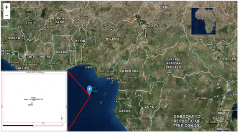
3.1 Location of study area
The study area is geographically located onshore Niger Delta within Latitude 5˚30I N and Longitude 6˚20I E (Figure 2). Five wells were drilled namely OS1, OS2, OS3, OS4 and OS5. However, after scrutinizing the dataset, the first three wells were selected for this study basically because they possess the log curve types required for the study (i.e. gamma ray, resistivity, sonic, neutron and density logs).
3.2 Geology of study area
The Niger Delta basin is an extensional rift basin in the Niger Delta region and the Gulf of Guinea on the passive continental margin near the western coast of Nigeria [22]. The clastic wedge of the Niger Delta occurs along a failed arm of a triple junction system that formerly emanated during the breakup that occurred between the South American and African plates.This process occurred in the late Jurassic crest [23, 24].
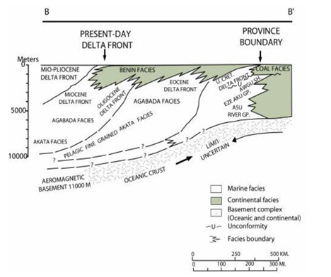
Figure 3 shows the stratigraphical column of the three formation types in the Niger Delta while Figure 4 is the cross section of the Niger Delta basin as modified by Whiteman [23].
Figure 2. A map showing the location of study area
Figure 3. A map showing the stratigraphy column with the three formation present in Niger Delta [22] modified by Doust and Omatsola [31]
Figure 4. A diagram showing the Southwest-Northeast (B-B’) cross section through the Niger Delta [23]
The age of the basin as defined by Klett et al. [25], extends from Eocene to Present. The delta had prograded southward, forming depobelts that accounts for one of the largest regressive deltas in the world with thickness of over 10km [26], an area of about 300,000km2 and a sediment volume of 500,000km3 [27, 28]. The petroleum system of the Niger Delta province is referred to as the Tertiary Niger Delta petroleum system [29] and it is divided into three litho-stratigraphic units [30].
First, the deep seated Akata Formation with thickness of about 6,400m at the center of the clastic wedge. This overpressured, ductile dark marine shale and silt with streaks of sand (turbidite flow origin) is the source rock unit. The age of the Akata Formation ranges from Paleocene to Recent and grades vertically into the overlying Agbada Formation [31]. The second formation is the Agbada Formation. It is known as the major hydrocarbon bearing (reservoir) unit consisting of paralic siliclastics, basically sandstone with intercalation of shale. Agbada Formation is further overlaid by the Benin Formation. This formation is characterized by poorly sorted, medium to fine grained radioactive marine sands and gravels with vestiges of shale. The structural features present in the Niger Delta also serves as the trapping mechanisms, they include, simple rollover structures with clay filled channel, growth faults, antithetic fault and collapsed crest [24].
According to the geology of the Niger Delta, which is the study area, there are three formation type (i.e. Benin, Agbada and Akata Formations). Since most well logs are hydrocarbon exploration oriented and Agbada formation has proven to be the location of interest (reservoirs bearing units). The available wells logs were observed to cover this formation. Therefore, this study is mainly focused on the Agbada Formation of the Niger Delta.
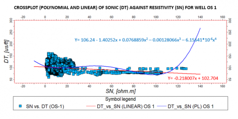
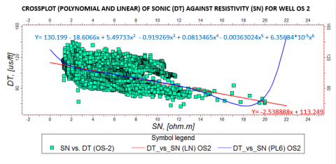
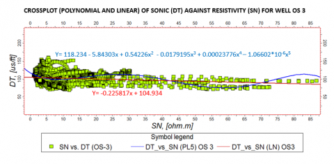
The general cross-plots of sonic against resistivity for well OS1, OS2 and OS3 are displayed in Figure 5, Figure 6 and Figure 7 respectively. The equation of the line of best fit for each cross-plot were used to transform resistivity into pseudo sonic logs for the wells.
Figure 5. Linear and Polynomial cross-plot of sonic (DT) against resistivity (SN) for well OS1
Figure 6. Linear and Polynomial cross-plot of sonic (DT) against resistivity (SN) for well OS2
Figure 7. Linear and Polynomial cross-plot of sonic (DT) against resistivity (SN) for well OS3
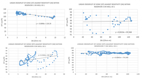
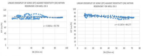
Figure 8 and Figure 9 shows the cross-plots of sonic against resistivity SN for previously delineated gas bearing units of wells OS1 and OS3 respectively. These cross-plots in Figure 8 show some scattered data which were expected due to the difference in response of the two log types in the presence of gas. A linear equation of the line of best-fit was utilized to get a better relationship between the logs in these gas zones and a linear equation was established.
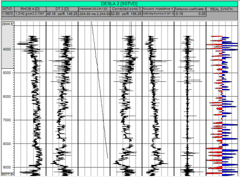
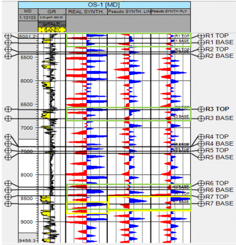
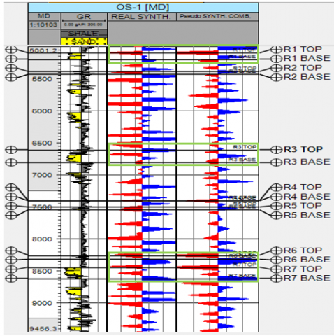
Figure 10 reveals the lithology and synthetic seismogram generated for well OS1. Track 1 is the lithology log, track 2 shows the standard synthetic seismogram generated with sonic and density logs, track 3 is the linearly generated general pseudo synthetic seismogram while track 4 is the pseudo-synthetic seismogram created with the polynomial transformed pseudo-sonic log. Figure 11 also shows the lithology and synthetic seismograms of well OS1, but this time we have the standard synthetic seismogram on track 2, placed side by side with pseudo-synthetic generated using the combined spliced pseudo-sonic log on track 3.
The region covered in green boxes are delineated gas zones while the areas covered in yellow boxes are regions with observed depth shift.
Although, some minor differences in depth and polarity as identified with the yellow boxes in Figure 10 occur between the standard synthetic and the other two pseudo synthetics (linear and polynomial). There exists a fair correlation across the wells apart from the obvious disparities observed with reservoirs 1, 3, 6 and 7 which corresponds to the previously delineated gas zones. Figure 11 which shows the standard synthetic and the combined-spliced pseudo synthetic reveals better general correlation across the reservoirs in these intervals. The disparities seen on the two previously generated pseudo synthetic that do not account for the effect of gas were absent in the combined spliced synthetic.
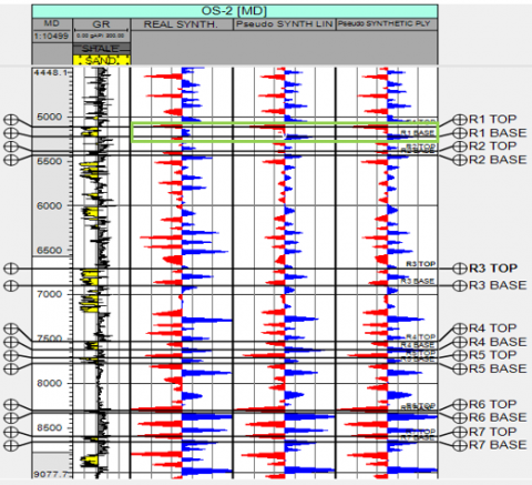
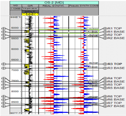
Figure 12 shows the lithology and synthetic seismogram generated for well OS2. Track 1 is the lithology log, track 2 is the standard synthetic seismogram generated with sonic and density log, the third tack shows the linearly generated general pseudo-synthetic seismogram and finally track 4 reveals the pseudo-synthetic seismogram created with the transformed polynomial transformed pseudo-sonic and density logs. Figure 13 shows the lithology and synthetic seismograms, but this time we have the standard synthetic seismogram on track 2 followed by the pseudo-synthetic generated using the combined spliced pseudo-sonic log on track 3.
Figure 8. Linear cross-plot of gas saturated region in OS1
Figure 9. Linear cross-plot of gas saturated region in OS3
Figure 10. Synthetic seismogram of well OS1 (Track 1 is the lithology log GR, track 2 is the standard synthetic seismogram created with the sonic and density log, track 3 is the pseudo-synthetic seismogram generated with the linear pseudo-sonic log, and track 4 represents the polynomial generated pseudo-synthetic seismogram)
Figure 11. Synthetic seismogram of well OS1 (Track 1 is the Gamma ray lithology log, track 2 represents the standard synthetic seismogram while track 3 shows the combined spliced pseudo-synthetic seismogram)
All the reservoirs delineated in well OS2 were oil saturated. As seen in Figure 10, a fairer general correlation was observed in these zones. Although, none of the reservoirs is gas saturated, the crossplot for reservoir 1 was seen to have some scattered data, which might be as a result of the hole conditions as observed and noted by the loggers. As revealed in Figure 13, combined spliced pseudo synthetic was also generated for reservoir 1 as indicated with the green box to correct this anomaly. The result shows a better correlation as it was able to correct the anomaly observed in Figure 12. Depth shift was not observed on Well OS2. However, difference in signal amplitude were observed in some units
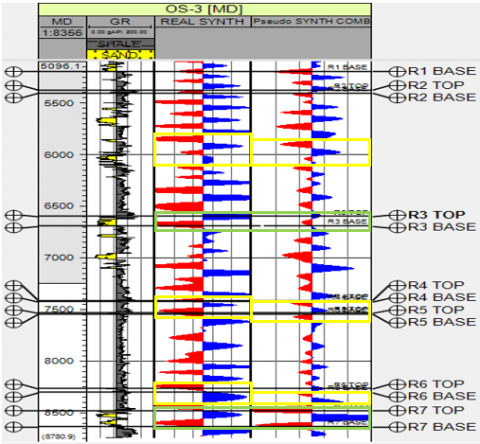
Figure 14 shows the lithology and synthetic seismogram for well OS3. Track 1 is the lithology log, track 2 shows the standard synthetic seismogram generated with sonic and density log, track 3 is the linearly generated general pseudo-synthetic seismogram while track 4 is the pseudo-synthetic seismogram created with the transformed polynomial transformed pseudo-sonic and density logs. Figure 15 shows the lithology and synthetic seismograms, but this time we have the standard synthetic seismogram on track 2 placed side by side with pseudo synthetic generated using the combined spliced pseudo-sonic log on track 3.
As seen in Figure 14, most of the reservoirs on well OS3 are oil saturated except reservoirs 3 and 7 which were gas saturated. Apart from the depth shift as marked with yellow boxes, a fair correlation was observed between the standard synthetic and the other two pseudo synthetics (linear and polynomial generated). However, the gas saturated zones appear otherwise.
Although some minor disparities in amplitude signals and the depth shift observed in Figure 14 persists. The combined spliced pseudo synthetic on track 3 in Figure 15 shows better correlation when compared with the control.
The observed slight difference in depth might be as a result of dispersion in seismic wavelet utilized during the process of generating the synthetic seismograms. Although, sonic log and resistivity log can both be used in calculating the porosity of a formation. It is important to acknowledge the fact that these two log types measure different physical properties in a formation (i.e. resistivity measures electric current flow, while sonic log works with rate of interval transit time in various geologic units).
Figure 12. Synthetic seismogram of well OS2 (Track 1 is the lithology log (GR), track 2 is the standard synthetic seismogram created with the sonic and density log, track 3 is the pseudo-synthetic seismogram generated with the linear pseudo-sonic log, and track 4 represents the polynomial generated pseudo-synthetic seismogram)
Figure 13. Synthetic seismogram of well OS2 (Track 1 is the Gamma ray lithology log, track 2 represents the standard synthetic seismogram while track 3 shows the combined spliced pseudo-synthetic seismogram)
Figure 14. Synthetic seismogram of well OS3 (Track 1 is the lithology log (GR), track 2 is the standard synthetic seismogram created with the sonic and density log, track 3 is the pseudo-synthetic seismogram generated with the linear pseudo-sonic log, and track 4 represents the polynomial generated pseudo-synthetic seismogram)
Figure 15. Synthetic seismogram of well OS3 (Track 1 is the Gamma ray lithology log, track 2 represents the standard synthetic seismogram while track 3 shows the combined spliced pseudo-synthetic seismogram)
The methodology utilized for this study will help to improve the mundane transformation techniques especially for siliclastics reservoirs with presence of gas. From the result, the correlation between the standard synthetic seismogram and combined spliced pseudo synthetic seismogram that considered the effect of gas is seen to be fair. This established relationship between resistivity and sonic logs can help to complement and enhance interpretation of data in fields with absence of sonic logs as a result of one reason or the other.
Rudman [32] noted that out of 15,000 wells drilled in the Indiana, less than 1,000 wells had CVL (continuous velocity logs), which were used for the generation of synthetics.
Whereas, Resistivity logs were observed to be present in most wells. Having a way to generate pseudo sonic log in wells where sonic log is absent can help to further enhance data interpretation in such fields. However, it is good to note that, the resistivity logs to be utilized for this transformation must be chosen carefully as discussed previously.
Furthermore, in cases where the quality of seismic is poor and stacking velocity is not easily retractable, the combined spliced pseudo-synthetic seismogram generated through this approach can be useful in data processing and modeling. It can also be utilized to validate the outcomes of prior synthetic seismogram generated during interpretation especially within zones with loose materials and gas saturated zones, which might have reduced the quality of recorded acoustic signals.
[1] Schlumberger (1989) Log Interpretation: Principles/Applications. Schlumberger Wireline and Testing. 225 Schlumberger Drive, Sugar Land, Texas No. 77478.
[2] Abe, S.J., Ayuk, M.A., Mogaji, A., Kafisanwo, O.O. (2018). 3D spatial distribution of reservoir parameters for prospect identification in ''Bizzy'' field, Niger Delta. Research Journal of Environmental and Earth Sciences, 10(1): 24-33. https://doi.org/10.19026/rjees.10.5864
[3] Haldersen, H., Dasleth, E. (1993). Challenges in reservoir characterization: GEOHORIZONS. American Association of Petroleum Geologists Bulletin, 77(4): 541-551.
[4] Acvedo, H., Pennington, W.D. (2003). Porosity and lithology prediction of caballos formation in Puerto colon oil field in Putumayo (Caballos). The Leading Edge, 22(11): 1134. https://doi.org/10.1190/1.1634919
[5] Faust, L.Y. (1951). Seismic velocity as a function of depth and Geological time. Geophysics, 16(2): 192. https://doi.org/10.1190/1.1437658
[6] Quadir, A., Lewis, C., Rau, R.J. (2018). Generation of Pseudo synthetic seismograms from Gamma-Ray well logs of high radioactive formations. Pure and Applied Geophysics, 176(4): 1579-1599. https://dx.doi.org/10.1007/s00024-018-1979-6
[7] Kung, S.L., Lewis, C., Wu, J.C. (2013). A technique for improving pseudo-synthetic seismograms generated from neutron logs in gas saturated clastic rocks. Journal of Geophysics and Engineering, 10(3): 035015. https://doi.org/10.1088/1742-2132/10/3/035015
[8] Dos Santos, W.L.B., Ulrych, T.T., De Lima, O.A. (1988). A new approach for deriving pseudo-velocity log from resistivity logs. Geophysical Prospecting, 36(1): 83-91. https://doi.org/10.1111/j.1365-2478.1988.tb02151.x
[9] Lee, M.W. (1999). Methods of generating synthetic acoustic logs from resistivity logs of gas-hydrates bearing sediments. U.S Geological Survey Bulletin. https://doi.org/10.3133/b2170
[10] Faust, L.Y. (1953). A velocity function including lithologic variation. Society of Exploration Geophysicist, 18(2): 271-288. https://doi.org/10.1190/1.1437869
[11] Kim, D.Y. (1964). Synthetic velocity log. 33rd Annual International Meeting, New Orleans.
[12] Alberty, M. (1994). The influence of the borehole environment upon compressional sonic logs. SPWLA 35th Annual logging Symp., 37(4).
[13] Kung, S.L., Lewis, C. (2014). A resistivity log-derived and gas-corrected pseudo-synthetic seismogram: application to the Fanpokeng Gas Field of north-western Taiwan. New Zealand Journal of Geology and Geophysics, 57(1): 21-31. https://doi.org/10.1080/00288306.2013.839454
[14] Telford, W.M., Geldart, L.P., Sheriff, R.E. (1990). Applied Geophysics (Second Edition). Cambridge University Press.
[15] Omuvwie, U., Tummala, R. (2009). Impact of borehole washout on acoustic logs and well-to-seismic tie. Society of Petroleum Engineers. Nigeria Annual International Conference and Exhibition, Abuja, Nigeria. https://doi.org/10.2118/128346-MS
[16] Asquit, G., Krygowski, D. (1982). Basic well log analysis. American Association of Petroleum Geologists, 16: 9. https://doi.org/10.1306/Mth16823
[17] Anderson, P., Newrick, R. (2008). Strange but true stories of synthetic seismogram. Canadian Society of Exploration Geophysicists, 33(10).
[18] Akinsete, O.O., Adekoya, D.A. (2016). Effects of mud filtrate invasion on well log measurements. Society of Petroleum Engineers, SPE-184308-MS. https://doi.org/10.2118/184308-MS
[19] Satoshi, I., Koji, N. (1996). The relationship between velocity and porosity of rocks with the effect of clay minerals. Journal of Japanese Association for Petroleum Technology, 61(3): 239-245. https://doi.org/10.3720/japt.61.239
[20] Nabway, B.S., Kassab, M.A. (2014). Porosity-reducing and porosity-enhancing diagenetic factor for some carbonate microfacies: a guide for petrophysical facies discrimination. Arabian Journal of Geosciences, 7: 4523-4539. https://doi.org/10.1007/s12517-013-1083-2
[21] Hacikoylu, P., Dvorkin, J., Mavko, G. (2006). Link between electrical resistivity and seismic velocity. 68th EAGE Conference and Exhibition Incorporating SPE EUROPE 2006. http://doi.org/10.3997/2214-4609.201402262
[22] Tuttle, M.L.W., Charpentier, R.R., Brownfield, M.E. (1990). The Niger Delta Petroleum System: Niger Delta Province, Nigeria, Cameroon, and Equatorial Guinea, Africa. CERT Logo, U. S. Department of the Interior, U.S. Geological Survey.
[23] Whiteman, A (1982). Nigeria: its Petroleum Geology, Resources and Potential. Graham and Trotman, London.
[24] Evamy, B.D., Harembourne, J., Kamerling, P., Knaap, W.A., Molley, F.A., Rowlands, P.H. (1978). Hydrocarbon habitat of the Tertiary Niger Delta. American Association of Petroleum Geologists Bulletin, 62: 1-39. https://doi.org/10.1306/M35439C19
[25] Klett, T.R., Ahlbrandt, T.S., Schmoker, J.W., Dolton, J.L. (1997). Ranking of the world‘s oil and gas provinces by known petroleum volumes. U.S. Department of the Interior Geological Survey, 97-463. https://doi.org/10.3133/ofr97463
[26] Kaplan, A., Lusser, C.U., Norton, I.O. (1994). Tectonic map of the world, panel 10: Tulsa, American Association of Petroleum Geologists, scale 1:10,000,000.
[27] Kulke, H. (1995) Regional Petroleum Geology of the World. Part II: Africa, America, Australia and Antarctica. Lubrecht & Cramer Ltd., Berlin, 143-172.
[28] Hosper, J. (1965). Gravity field and structure of Niger Delta, Nigeria, West Africa. Geology Society of American Bulletin, 76(4): 407-422. http://doi.org/10.1130/0016-7606(1965)76[407:GFASOT]2.0.CO;2
[29] Avbovbo, A.A. (1978). Tertiary lithostratigraphy of Niger Delta1. American Association of Petroleum Geologists Bulletin, 62(2): 295-300. https://doi.org/10.1306/C1EA482E-16C9-11D7-8645000102C1865D
[30] Weber, K.J. (1987). Hydrocarbon distribution pattern in Nigerian growth fault structures controlled structural style and stratigraphy. J. Petrol Sci Eng., 1(): 1-12. https://doi.org/ 10.1016/0920-4105(87)90001-5
[31] Doust, H., Omatsola, M. (1990). Petroleum geology of the Niger delta. Geological Society, London, Special Publications, 50(1): 365-365. https://doi.org/10.1144/GSL.SP.1990.050.01.21
[32] Rudman, A.J. (1982). Interrelationship of resistivity and velocity logs. Developments in Geophysical Exploration Methods-3, 33-59. https://doi.org/10.1007/978-94-009-7349-7_2