Tarek Houari | Mohamed Benguediab* | Azzeddine Belaziz | Tayeb Kebir
© 2020 IIETA. This article is published by IIETA and is licensed under the CC BY 4.0 license (http://creativecommons.org/licenses/by/4.0/).
OPEN ACCESS
In the present paper, we propose a numerical modeling of fracture behavior of High Density Polyethylene (HDPE) using different fracture mechanics approaches as well as a simulation of the static behavior by calibrating the static traction curves in order to highlight the feasibility of the model in reproducing the results of the EWF. The numerical determination of the fracture parameters by the global approach which will be validated by a simulation by means of DENT specimens and results obtained are compared to those of experimental results.
HDPE, fracture mechanics, EWF, J integral, GTN, global approach, local approach, Abaqus
The development of structural polymers is linked to their mechanical properties, which themselves depend on the microstructure, accordingly semi-crystalline polymers have for the most part a high tenacity that meets the requirements of products which must necessarily withstand severe conditions of use such as (impact, creep, fatigue). Among these materials HDPE which is most widely used particularly in urban water distribution networks and those for the distribution of natural gas. Damage or presence of cracks in such pipes can lead to leaks which are harmful both to financial and environmental terms and to some extent a sudden rupture may have more serious consequences.
Determining the fracture strength of these materials is a main objective of either users or manufacturers. Arguably several authors have tried to understand the mechanisms of failure of thermoplastic materials [1-5]. Fracture mechanics concepts are of important use to characterize the fracture mechanical behavior occurring at stresses lower than the material elastic limit, under these conditions it is considered that plasticity at the tip of the crack is confined and the process of rupture has a brittle nature. In this condition, fracture parameter such as Critical Stress Intensity Factor, KIc or the critical strain energy release rate, GIc are used to characterize this type of fracture. During the 1970s, numerous studies were centered on the search for a parameter that can extend fracture mechanics to the elastoplastic behavior of materials [6, 7].
Among the different parameters, the J integral concept developed by Rice [8] which has very successful due to its ease of implementation and the numerical properties, having an energy obtained by a simple contour integral, independent of it. Begley and Landes [9] associated the integral J with a priming criterion Jc (J critical), which was later extended to ductile propagation via the tear resistance curves J - Δa.
Wells [10] then Burdekin et al. [11], used the spacing of the two surfaces at the bottom of crack (CTOD: Crack Tip Opening Displacement) so as to study of a crack the behavior. The concept of essential work of fracture has also been proposed by Broberg [12] as an alternative to the integral J approach when the materials are ductile.
Besides to what was said above, another approach called local has been developed to understand the mechanisms of failure of materials. This approach is based on the modeling of damage by a mechanism of germination, growth and coalescence of cavities born on second phase inclusions. Several models have been developed to describe the growth of cavities.
The most widespread model is that of Rice and Tracey [13] who considered a spherical cavity in an infinite medium made of a rigid plastic material. Coalescence appears when R / Ro ratio reaches a critical value (R / Ro)c.
Other models also have been developed and are based on the volume density of cavities which is a determining parameter for the characterization of ductile rupture. Among these models, we can cite that of Rousselier [14] and Gurson [15]. Accordingly, Tvergaard and Needleman have integrated the coalescence and the germination of the cavities in the Gurson model [16], which at endproduced the Gurson-Tvergaard-Needleman (GTN) model.
Further, numerical simulations based on the Gurson-Tvergaard-Needleman (GTN) model already presented. Their application to HDPE will allow us to compare this type of approach with the experimental data. A simulation of the static behavior by calibrating the static traction curves in order to highlight the feasibility of the model in reproducing the results of the EWF. To determine the fracture parameters by the global approach we use a numerical simulation on DENT specimens [17].
2.1 Study material
In this work, the material used is high-density polyethylene (HDPE). It is a semi-crystalline thermoplastic widely used in engineering applications such as pipelines and pressure vessels [18].
2.2 Numerical model of the tensile specimens
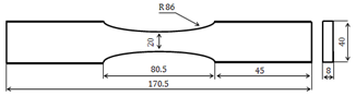
For simulation of the tensile specimens in FEM code, we use a software code ABAQUS/CAE function [19], a geometric model of the tensile specimens is produced, with the consideration of symmetry, it is modeled only half of the specimens shown in Figure 1.
The equations of the GTN model are implemented on the ABAQUS. The Gurson Tvergaard–Needleman (GTN) model, as is shown in Eq. (1).
$\phi \text{=}\frac{\sigma _{eq}^{2}}{\sigma _{0}^{2}}+2{{q}_{1}}{{f}^{*}}\cosh (\frac{3{{q}_{2}}{{\sigma }_{m}}}{{2{\sigma }_{0}}})-(1+{{({{q}_{1}}{{f}^{*}})}^{2}})=0$ (1)
where,
σeq is von Mises equivalent stress,
σ0 is the microscopic yield stress of the undamaged matrix material,
σm is the mean normal stress,
q1 and q2 are constitutive parameters introduced by Tvergaard to modify the original Gurson model.
Figure 1. Half geometry model of tensile specimen
2.3 Mechanical behavior model
To modeling the behavior of the material, we adopted an elastoplastic behavior model coupled with a damage model known as the porous plastic metals. The rupture simulation was carried out by a rupture criterion integrated in the GTN model; these criteria are the critical void volume fraction and the volume fraction at rupture.
The elastic part is materialized by the modulus of elasticity and the Poisson’s ratio. The plastic work hardening part is introduced point by point in the calculation code from the traction curve in Figure 2 [20].
The parameters of the GTN model are calibrated by trial and error until an acceptable correlation is obtained with the experimental traction curves.
Table 1. GTN parameters for the different calibrations
|
Tests |
Variables |
|||
|
|
q1 |
q2 |
fc |
fF |
|
A |
1 |
1.5 |
0.5 |
0.55 |
|
B |
1 |
0.8 |
0.5 |
0.55 |
|
C |
1.37 |
1.3 |
0.5 |
0.55 |
The consideration of the damage in the numerical model is guaranteed by the implementation of the GTN model included in all the models of porous metals. The Table 1 summarizes the parameters used for the calibration of our material. In this modeling q3 is taken equal to q12.
Figure 2. Stress-strain curves [20]
2.4 Mesh and boundaries conditions
2.4.1 Tensile specimens
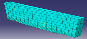
The 2D finite element model geometry with 154 elements, in which the type of element used in static mechanical behavior analysis is a linear quadrilateral elements of plane stress type with reduced CPS4R integration.
The Figure 3 illustrates the finite element mesh adopted for the numerical simulation of static mechanical behavior.
The boundary conditions applied to the tensile specimen are: a displacement and a rotation (U2 = UR2 = 0) along the Y axis. The application of the symmetry model FE on the X axis is chosen for the reduction of the calculation time.
Figure 3. Finite elements mesh of the tensile specimens
2.4.2 DENT specimens
In the simulation of the EWF tests, the DENT specimens were modeled in 3 dimensions, the Figure 4 represents the adopted mesh.
Figure 4. Finite element mesh of the DENT specimens
The choice of the mesh is important for two reasons which guide its dimensioning. On the one hand, the greater the number of degrees of freedom, the longer the calculation time.
On the other hand, the impact of the mesh which is linked to the precision of the desired result. This means that the smaller the elements, the more the solution announced by the solver approaches the appropriate solution. The element type selected is C3D8R (element eight first order nodes with reduced integration). The boundary conditions are set as follows: the edge of the specimen following the X axis is considered to be XSYMM (U1 = UR2 = UR3 = 0).
2.4.3 CT specimens
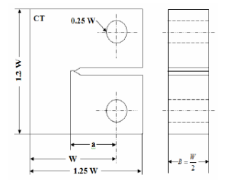
As it was introduced in the preceding chapter, the characterization of the resistance to rupture by the approach of the J integral contour is carried out on CT specimens (Compact Tension). Several authors have used this type of specimens in the literature [21]. The Figure 5 shows the geometry of this specimen. The contour integral is calculated by the Eq. (2):
$J=\frac{\eta U}{B\left(W-a_{0}\right)}$ (2)
The Merkle-Corten parameter η for CT specimens is equal to (2 + 0.522 (b0/W)) where b0 is the length of the uncracked ligament W-a0. The Eq. (2) therefore becomes:
$J=\frac{\left(2+0.522 \frac{b_{0}}{W}\right) U}{B\left(W-a_{0}\right)}$ (3)
Figure 5. Geometry of CT specimens
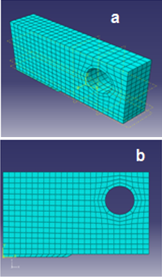
Figure 6. EF CT models in (a) 3D and (b) 2 D
Figures 6.a and 6.b represent the geometric models in finite elements three and two dimensions respectively.
3.1 Mechanical behavior model
After several tests and calibrations, the parameters of the GTN model are calibrated by adjusting the numerical results until an acceptable correlation is obtained with the experimental traction curves. The Figure 7 clearly illustrates the effect of chosen parameters from the GTN model.
The symbols indicate the parameters used according to Table 1. In Figure 7, it is the curve C which best correlates with the experimental curve [20]. So, these are the parameters of test C that we will use for the simulation of the DENT specimens rupture.
Figure 7. Stress-strain curves of the different simulations compared to experimental results [20]
Figure 8 represents the different stages of Von Mises stresses and plastic deformations with the volume fractions of the voids during the loading of the tensile specimens.
Figure 8. The different stage of Von Mises stresses and Plastic deformations
3.2 Simulation of EWF tests
The ligament lengths used in this study are 7, 9, 11, 13, 15, 17, 25 and 33 mm. in which lengths are chosen in order to compare our results with those of Houari et al. [20]. The different geometric models are presented in Figure 9.
Figure 9. Some DENT models in symmetry
3.3 Fracture behavior analysis
In this part, the analysis of the numerical modeling results of the DENT specimens were presented and checked the conditions of the EWF concept and then validate the results by experimental comparison.
3.3.1 Analysis of the conditions of the EWF method
One of the necessary conditions for the validation of the EWF method is the plastic zone around the ligament, since condition has been checked to ensure the condition of the plane stresses.
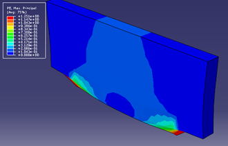
The analysis of the results of the different simulations shows that the ligament length is fully plasticized before the start of the void initiation process. This is shown in Figure 10, where the plastic area surrounds the ligament.
Figure 10 clearly illustrates that the entire ligament is plasticized. The shape of this plastic zone is almost elliptical which well agrees with our experimental observations.
Figure 10. Plastic area around the ligament
For longer ligament lengths, after noting the appearance of edge effects, it appears that the mode of deformation is different as shown in Figure 11 for L = 33 mm. We notice a more pronounced curvature of the specimens at the two edges of the notch.
Figure 11. Plastic area for a high ligament L = 33 mm (Edge effect)
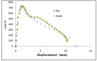
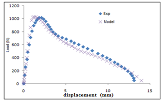
The Figures 12 and 13 present the results of the modeling of the load curves according to displacements.
The results are in accordance with our model compared to experimental results [20].
This consolidates the choice of parameters for the GTN model. The three zones of the damage process are representing an acceptable overlap with the experimental curves obtained by the EWF tests.
Figure 12. Curve load-displacement for ligament L=7 mm
Figure 13. Curve load-displacement for ligament L=9 mm
The shape of these curves confirms a ductile rupture for this type of polymer material with plasticization ligament. This shows that the mode of rupture is independent of the length of the ligament.
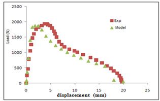
The load-displacement curves for the different ligament lengths chosen are presented in Figures 14a to 14e.
(a) Curve load-displacement ligament L=11 mm
(b) Curve load-displacement ligament L=13 mm
(c) Curve load-displacement ligament L=13 mm
(d) Curve load-displacement ligament L=15 mm
(e) Curve load-displacement ligament L=33 mm
Figure 14. Curve load-displacement for different lengths of ligament
As it has been previously estimated, DENT specimens with short ligament lengths give closer results to the experimental.
As the length increases, the modeled curves deviate more and more from the EWF test curves. This finding confirms the results and observations mentioned in the literature [20, 22].
5.1 Geometry models
According to standard ASTM E399 [23] for CT specimens the crack length (a) must meet the following double conditions:
$0.45 \leq \frac{a}{W} \leq 0.55$ (4)
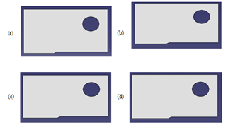
In this regard, we have modeled CT specimens in 2D with the ratios a/W (see Figure 6) 0.55, 0.53, 0.5, 0.47 and 0.45. The Figures 15 a-d represents the different lengths of crack studied numerically in Abaqus/CAE, respectively.
Figure 15. CT models analyzed numerically (a) a/W=0.55, (b) a/W= 0.53, (c) a/W= 0.5 et (d) a/W=0.47
5.2 Boundaries conditions and mesh
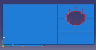
In order to guarantee a similarity between the experimental conditions and the numerical simulation we imposed a displacement on the axes level of the specimens fixation modeled by the holes on Figures 16. The Figure 17 illustrates the boundary conditions used in this analysis.
The Figure 17 illustrates the conditions for displacement imposed on the periphery of the specimen hole simulating the displacement of the fixing axes of the specimens.
Figure 16. Boundary conditions imposed on the symmetrical CT model
Figure 17. Representation of the displacement imposed on the specimen hole
5.3 Behavior analysis
The various stages of behavior for the various crack lengths are presented. The fields of deformation and stresses in the vicinity of the crack are analyzed.
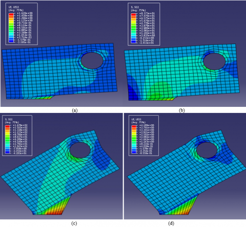
Figures 18 (a), (b) and (c) represent the iso values for an increment of displacement of 10% (0.1), it is noted that the stresses or centered in the crack point, the specimens are in a state of compression on the edges of the line on the crack plane.
This is illustrated by negative deformations on the edges of the hole and the lower left edge on the crack plane (Figure 18(c)).
Figure 18. Iso values of (a) displacement (b) stresses (c) deformations, for a displacement increment of 0.1
When pursuing the imposed displacements, we noticed an intensification of the stresses around the crack point. Displacements are negative above the uncracked ligament, which is reflected by compressions in this area. The different increments are brought together in Figures 19 (a), (b), (c) and (d).
Figure 19. Iso values of the stresses and strains for increments of displacement to 50% (a and b) et 100% (c and d)
5.4 J integral and numerical determination of Jc
5.4.1 Load-displacement curves
For the calculation of the energy parameter J, it is first necessary to obtain the Load curves as a function of the displacements. By studying the results of the forces as a function of the displacements for the different ligament lengths in the CT specimens, we will able to calculate the critical initiation energy which corresponds to the maximum load in the displacement forces curves.
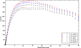
Figure 20 summarizes all the curves obtained numerically; by calculating the nodal reaction forces on the line of the uncracked ligament.
Figure 20. Load-displacement numerical curves for the analyzed 5 CT models
We noted that the maximum load increases with the increase in the non-cracked ligament. An interesting observation concerns the displacements which correspond to the maximum loads, further we noticed approximately the same value for all the ratios a/W. We can say that, it is necessary to predict a value of J equal of the critical value of initiation of the crack propagation.
5.4.2 Correlation between J integral and Load-Displacement curves
According to the literature [24], the authors noted that it is wise consider the value of J corresponding to the maximum load JM considered as a critical value. Figure 21. shows the obtained JM values for the different a/W ratios. It is noted that the value of JM is independent of crack the length. However, for different geometries such as SENB used in three-point bending, the authors confirm a distance between the results of JM; which means the inconvenience of the J approach for Polymer cases [24]. Regarding this study, we took the initiative to only calculate JC on a qualitative basis. Figure 22 illustrate the method adopted for determining JC for a/W=0.5.
Figure 21. Correlation of the value of J with the load as a function of displacements and determination of JC (a/W=0.5)
Figure 22. Numerical JC values depending on function of ligament lengths and the determination of JC average
Figure 22 summarizes the values of JC obtained for the various a/W ratios, we noticed that JC is independent of the crack length.
The results obtained are in good agreement with results obtained by Elmeguenni et al. [24].
In the research presented in this paper, the objective of this study has been extended to the relevance of fracture mechanics concepts on highly deformable materials, we used local approaches based on continuum damage mechanics, could be an alternative way to enrich the understanding of fracture of such materials.
In this context, the EWF concept can be present an alternative or a complementarily to the approach based on the integral J to determine the breaking strength properties of deformable materials.
- The constitutive model of Gurson-Tvergaard-Needleman is introduced in the finite element analysis to describe the behavior at quasi static loading and at rupture of the DENT test specimens of high HDPE-100. The parameters q1 and q2 have a significant influence on the tensile strength. The GTN model allows a good calibration of the parameters and allows a modeling of the real behavior by the finite element method.
- The coupling of the GTN model as a damage model with the elastoplastic behavior taken as the traction curve true stresses as a function of true deformation, allows us to characterize our material, HDPE, at rupture.
- The EWF method can be performed numerically for the characterization of the We parameter or the essential work of fracture.
- The determination of critical J based on the correlation between the numerical values of J and the Load curves as a function of the displacements calculate on CT test pieces used for the experimental.
- The EWF method, by its simplicity, is the most suitable for characterizing the parameter of the intrinsic failure of the material.
This work is carried out in the laboratory of reactive materials and systems which is sponsored by the direction of scientific and technological research DGRST.
[1] Marshall, G.P., Culver, L.E., Williams, J.G. (1970). Craze growth in poly(methylmethacrylate): A fracture mechanics approach. Proceedings of the Royal Society of London. Series A, Mathematical and Physical Sciences, 319(1537): 165–187.
[2] Tonyali, K., Brown, H.R. (1986). On the applicability of linear elastic fracture mechanics to environmental stress cracking of low density polyethylene. Journal of Materials Science, 21: 3116–3124. http://dx.doi.org/10.1007/BF00553345
[3] Allwood, W.J., Beech, S.H. (1993). The development of the ‘notched pipe test’ for the assessment of the slow crack growth resistance of polyethylene pipe. Construction and Building Materials, 7(3): 157–162. http://dx.doi.org/10.1016/0950-0618(93)90053-F
[4] Beech, S.H., Channell, A.D., Rose, L.J. (1995). Slow crack growth performance assessment in polyethylene pipe. In: Proceedings of the 14th International Plastic Fuel Gas Pipe Symposium, American Gas Association, San Diego.
[5] Boot, J.C., Guan, Z.W., Toropova, I.L. (1996). Structural design of thin walled polyethylene pipe linings for water mains. Plastics, Rubber and Composites Processing and Applications, 25(4): 174-179.
[6] Shih, C.F., Lorenzi, H.G., Andrews, W.R. (1979). Studies on crack initiation and stable crack growth. in Elastic-Plastic Fracture, ed. J. Landes, J. Begley, and G. Clarke (West Conshohocken, PA: ASTM International, 1979), 65-120. https://doi.org/10.1520/STP35827S
[7] Kanninen, M.F., Rybicki, E.F., Stonesier, R.B., Broek, D., Rosenfield, A.R., Marscall, C.W., Hahn, G.T. (1979). Elastic-plastic fracture mechanics for two-dimensional stable crack growth and instability problems.in Elastic-Plastic Fracture, ed. J. Landes, J. Begley, and G. Clarke (West Conshohocken, PA: ASTM International, 1979), 121-150. https://doi.org/10.1520/STP35828S
[8] Rice, J.E. (1968). A path independent integral and the approximate analysis of strain Concentrations by notches and cracks. Journal of Applied Mechanics, 35(2): 379-386. https://doi.org/10.1115/1.3601206
[9] Begley, A., Landes, J.D. (1972). The J Integral as a Fracture Criterion. ASTM STP 514.Appeared in Fracture Toughness, proceedings of the 1971 National Symposium on Fracture Mechanics, Part II. University of Illinois, Urbana-Champaign, Illinois, pp. 1-20.
[10] Wells, A.A. (1963). Application of fracture mechanics at and beyond general yielding. British Welding Institute Journal, 10-11: 563-570.
[11] Burdekin, F.M., Stone, D.E.W. (1966). The crack opening displacement approach to fracture mechanics in yielding materials. Journal of Strain Analysis, 1(2): 145-153. https://doi.org/10.1243%2F03093247V012145
[12] Broberg, K.B. (1968). Critical review of some theories in fracture mechanics. International Journal of Fracture Mechanics, 4: 11-19. https://doi.org/10.1007/BF00189139
[13] Rice, J.R., Tracey, D.M. (1969). On the ductile enlargement of voids in triaxial stress fields. Journal of the Mechanics and Physics of Solids, 17(3): 201–217. https://doi.org/10.1016/0022-5096(69)90033-7
[14] Rousselier, G. (1987). Ductile fracture models and their potential in local approach of fracture. Nuclear Engineering and Design, 105(1): 97–111. http://dx.doi.org/10.1016/0029-5493(87)90234-2
[15] Gurson, A.L. (1976). Porous rigid-plastic materials containing rigid inclusions: yield function, Plastic potential, and void nucleation. US Energy Research and Development Administration (ERDA), United States.
[16] Tvergaard, V., Needleman, A. (1984). Analysis of the cup-cone fracture in a round tensile bar. Acta Metallurgica, 32(1): 157–169. https://doi.org/10.1016/0001-6160(84)90213-X
[17] ASTM E8. (2004). Standard Test Methods for Tension Testing of Metallic Materials. Part IA. Metals Mechanical Testing Elevated and Low Temperature Tests Metallograph., 3(1): 1–24.
[18] Azzeddine, B., Mazari, M. (2018). Experimental study of the weld bead zones of a high-density polyethylene pipe (HDPE). Journal of Failure Analysis and Prevention, 18: 667-676. https://doi.org/10.1007/s11668-018-0462-0
[19] Hibbitt, Karlsson, Sorensen. (1989). ABAQUS Example Problems Manual. Hibbitt, Karlsson & Sorenson, Inc.
[20] Houari, T., Benguediab, M., Belaziz, A., Belhamiani, M., Aid, A. (2020). Fracture toughness characterization of high density polyethylene using essential work of fracture concept. Journal Failure Analysis, 20: 315-322. https://doi.org/10.1007/s11668-020-00829-6
[21] Williams, J.G. (1984). Fracture mechanics of polymers. Polymer Engineering and Science, 17(3): 144-149. https://doi.org/10.1002/pen.760170303
[22] Elmeguenni, M. (2010). Effect of triaxiality on the behavior and rupture of high density polyethylene: experimental and numerical approaches. PhD Thesis, Lille1 University, Science and Technology, France.
[23] ASTME399. (1997). Standard test for plane-strain fracture toughness of metallic materials. Part IA. Metals Mechanical Testing Elevated and Low Temperature Tests Metallograph, 3(1): 1-31. https://doi.org/10.1520/E0399-90R97
[24] Elmeguenni, M., Naït-Abdelaziz, M., Zaïri, F., Gloaguen, J.M. (2013). Fracture characterization of high-density polyethylene pipe materials using the J-integral and essential work of fracture. International Journal of Fracture, 183: 119-133. https://doi.org/10.1007/s10704-013-9848-x