OPEN ACCESS
While traveling, the traveling detection pulse radar cannot capture the accurate target information through signal process, owing to the Doppler effect. To solve the problem, this paper attempts to design a proper compensation method into signal processing to correct the Doppler information of the target. Specifically, the existing signal processing algorithms of pulse radar were reviewed in details, namely, pulse compression, moving target detection (MTD) and constant false alarm rate (CFAR) detection). Based on the MTD and CFAR and considering the requirements of 3D geographic scene, the author developed a real-time calculation method of radar 3D detection range and 2D slice at specified altitude under terrain shading factor. After determining the target nature by the radar signals, the corresponding 3D model was adopted to realize a realistic display of the target, which verifies the effectiveness of the proposed method.
pulse radar, traveling detection, geographic scene, signal processing, speed compensation
The traveling detection requires a maneuverable radar structure and a rational signal processing algorithm. Typically, the adaptive anti-jamming algorithm (Malvezzi et al., 2011) and the compensation algorithms for speed, distance and beam (Meng et al., 2008) are adopted for traveling detection radar.
The compensation algorithms for traveling detection radar mainly acquire the latest attitude data (e.g. speed, course, pitch angle, roll angle, eastward speed, northward speed, and celestial speed) from the attitude navigation device of the radar, and revise the target parameters and the algorithm parameters. The general purpose of these algorithms is to provide the information of the radar, including but not limited to attitude, position and speed, quickly through the integrated navigation device (Becker, 1987), and complete the detection of the target information.
By the design plan, the existing compensation algorithms fall into three categories, namely, speed compensation, beam compensation and track compensation. Specifically, the speed compensation mainly makes up for the Doppler frequency of the target, thereby eliminating the Doppler distortion caused by the radar movement. Based on the instantaneous attitude of the radar, beam compensation corrects the direction of the radar transmitting beam, aiming to satisfy the tracking requirements and realize effective coverage of space. The track compensation compensates the distance and azimuth information of the target track, such that the target track can reflect the relative position of the vehicle in real time. The above three types of compensation algorithms work can effectively ensure the validity and authenticity of the data detected by a moving radar.
The traveling detection radar, which mainly works in low-altitude regions, faces many interferences in the 3D geographic scene. The interferences are particularly serious in the motion state, as the disturbance grows more complex and the clutter becomes dynamic in the changing environment. In this case, some of the Doppler information permeates into the static background clutter, and intermingles with the Doppler information of the real moving target, making it difficult to detect the target accurately. It is impossible to extract the effective target information if the interference or clutter is sufficiently powerful to submerge the echo signal of the moving target.
The popular techniques to realize anti-jamming detection include pulse compression, moving target detection, and constant false alarm rate (CFAR) detection (Antipov and Baldwinson, 2008). Here, the last two techniques are adopted to improve the anti-jamming ability of the traveling detection radar. For traditional pulse radar, the fast Fourier transform (FFT) (Fan et al., 2014) is often coupled with moving target detection to improve the processing speed and real-time performance. However, the ratio of main lobe to sidelobe (hereinafter referred to as the ML-SL ratio) of this approach is merely 13dB, failing to fulfill the target detection requirements under interference. In view of the above, this paper proposes a new filtering algorithm to improve the ML-SL ratio and the anti-jamming ability.
The processing of pulse radar signals consists of two key steps: signal sorting and sorted signal recognition. The signals are usually separated, divided and recognized according to multiple parameters. The most popular processing method is to sort and recognize radar signals based on prior knowledge and simple processing (Wang and Xi, 2003; Rui et al., 2002).
Much research has been done on radar signal sorting since the 1970s. The most representative sorting algorithms include sequential column search, multi-parameter clustering based on spatial distance, as well as box matching based on parameter quantization tolerance (He et al., 2009; Xiao et al., 2013).
The traditional sorting strategy for pulse radar signals can be divided into two phases: pre-sorting and primary sorting. In the pre-sorting phase, the signals are sorted by such information as carrier frequency, pulse width and angle of arrival. If the sorting fails, the signals will be sorted again by the arrival time of the pulse wave. However, the pre-sorted signals of a complex radar system cannot be sorted well by the traditional sorting algorithms.
Emerged in the 1980s, the pulse repetition interval (PRI) transform algorithm, a classic pulse radar signal sorting algorithm, enjoys good subharmonic suppression effect and works well for fixed and dithered repetition frequency pulse sequences. The PRI can transform the difference between pulse sequences into a spectrum, and estimate the value of each pulse sequence from the corresponding peak position.
Besides the PRI transform, many other methods have been developed to sort the signals of a complex radar system. For example, Wang (2011) put forward a radar signal sorting algorithm based on support vector analysis. Liu and Shi (2009) designed a fuzzy associative sorting algorithm for radar pulse signals on the basis of bidirectional associative memory (BAM) network and fuzzy theory. Guo et al. (2010) proposed a synthetic sorting method for radar pulse sequence. Ahmed and Tang introduced piecewise clustering method to pulse radar sorting processing. Montazer et al. (2013) improved the fuzzy C-means clustering algorithm with the ant colony algorithm
The recent vogue of the backpropagation (BP) neural network has aroused interests in sorting pulse radar signals with artificial intelligence algorithms. For instance, Du et al. (2010) developed a sorting algorithm of aerial radar signals based on multi-2D radial basis function (RBF) neural network, which can classify unknown data after proper training.
With the growing radar density in the environment, the amount of radar signals is continuously rising. It is now imperative to improve the computing efficiency of classical radar signal sorting algorithms which used to be efficient, such as statistical histogram, cumulative difference histogram and sequence difference histogram (Klilou et al., 2014).
Radio detection and ranging are the main functions of radar. To find and position a target in space, the radar needs to transmit a radio wave and receive the electromagnetic wave reflected back by the target. This section reviews some traveling detection techniques of pulse radar.
3.1. Echo signals of moving target
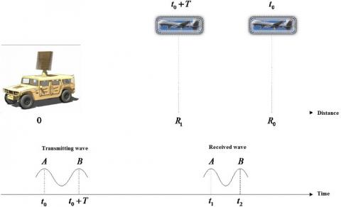
The pulse radar firstly transmits pulse signals for a period of time and then receives the echo signals reflected back by the target. After that, the echo signals are processed through multiple steps to determine the range, azimuth and speed of the target. The moving target detection (MTD) mainly relies on the Doppler effect (Figure 1) of moving targets: when there is a relative radial speed between the transmitter and the target, the frequency of the reflected signals of the target is different from that of the transmitted signals.
Figure 1. The doppler effect
The spatial relationship between the target distance R detected by radar and the transmission delay τ can be expressed as:
$R=\frac{c \tau}{2}$ (1)
where c is the propagation speed of electromagnetic wave in space. Let T (T=1⁄f, with f being the radar transmitting frequency) be the transmitting period of the radar, and v be the speed of the target moving towards the radar. As shown in Figure 1, when $t=t_{0},$ the radar transmitting wave peaks at point $A$ and the target distance from the radar is $R=R_{0} ;$ when $t=t_{0}+T,$ the radar transmitting wave peaks at point $B$ and the target distance from the radar is $R=R=R_{1} .$ Thus, the time $\Delta t$ when point $A$ of radar transmitting wave is transmitted to the target can be defined as:
$\Delta t=\frac{R}{c+v}$ (2)
Sincc $\Delta t$ is also the time for the wave to return to the radar from the target, the time when point A of radar transmitting wave returns to the radar, denoted as $t_1$, can be expressed as:
$t_{1}=t_{0}+2 \Delta t=t_{0}+\frac{2 R_{0}}{c+v}$ (3)
Similarly, the time when point $B$ of the transmitted wave, which is reflected by the target, returns to the radar, denoted as $t_{2},$ can be expressed as:
$t_{2}=t_{0}+T+\frac{2 R_{1}}{c+v}$ (4)
The received radar echoes form periodic $T^{\prime}$ echo signals between $t_{1}$ and $t_{2} :$
$T^{\prime}=t_{2}-t_{1}=T-\frac{2\left(R_{0}-R_{1}\right)}{c+v}$ (5)
It can be seen from the above formulas that the period of electromagnetic wave reflected by the moving target changes with that transmitted by the radar. In other words, the echo of moving target has a varying frequency, which is known as the Doppler effect.
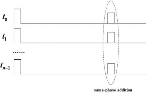
3.2. MTD and coherent accumulation
In the MTD, the fixed clutter should be removed from radar echo signals and the moving target should be detected by the principle of the Doppler effect. To improve the signal-to-noise ratio (SNR) of the target echo signals and enhance the detection ability of the target, the coherent accumulation is needed to stack the received signals in multiple radar transmission cycles with equal distance gates in the same phase.
Generally, MTD and coherent accumulation are implemented in a set of algorithms. Figure 2 provides an example to clearly illustrate the two concepts. Here, the distance between the moving target and the radar is assumed to be constant in successive transmitting cycles of the radar, so are the target echo of each transmitting pulse and the transmitting delay ($\Delta t$) in each successive period.
Figure 2. Transmitting and receiving schema of MTD pulse radar
The core idea of the MTD and coherent accumulation is to process the data in these periods and complete the same-phase addition in Figure 3.
Figure 3. Same-phase addition
For the same-phase addition of multiple pulse echo signals, a set of narrowband filters is needed to differentiate between Doppler frequencies. According to the Doppler effect, the Doppler frequency in the echo signals varies with the radial speed of the target. Since passband frequency is narrow and continuous, a dressing filter can be developed from many finite-impulse response (FIR) filters to accurately distinguish targets with different Doppler frequencies. The FIR filter bank can be designed as:
$\mathrm{y}(\mathrm{n})=\sum_{i=0}^{N-1} w_{i} x\left(n-i T_{r}\right)$ (6)
where $N$ is the number of filter coefficients; $T_{r}$ is the pulse repetition period; $n$ is a discrete time moment; $w_{i}$ are filter coefficients. The above formula can be explained as Figure 4 below.
Figure 4. Structure of MTD for FIR filter bank
3.3. CFAR detection
According to the principle of Doppler effect, the motion of the radar will inevitably cause the Doppler effect of stationary objects, creating a large number of false targets. This calls for Doppler correction (speed compensation) of detected targets before signal processing. Because of the changing attitude of the radar, the direction of radar transmitting beam will deviate from the expected direction. In this case, beam correction (beam compensation) is necessary for accurate measurement and tracking of the altitude. As the radar position changes during traveling, the origin of radar coordinate system will move, and the previous track will become inaccurate. Thus, the position of track information should be corrected (track compensation) to identify the position of track of target relative to the radar. The most direct solution is to install a complete navigation and attitude system on the moving radar, which can provide comprehensive and reliable attitude information for the signal processing system.
Based on the instantaneous data on radar attitude angle, the author adopted the beam compensation algorithm to ensure the space coverage of the radar in an inclined state, so that the radar will not miss any target in the space. The beam compensation is realized through the following steps. Firstly, the coordinates (R, A, E) in radar coordinate system was converted to geodetic coordinate system, where A is radar azimuth, E is the required pitch directioms $\varphi$ and R is a reference coefficient with no impact on the calculation results. Secondly, the transformation from geodetic coordinate system to radar coordinate system was carried out, yielding the coordinates $\left(R^{\prime}, A^{\prime}, \emptyset^{\prime}\right)$ of radar coordinate system. Finally, the correction amount of the current beam transmitting angle was calculated as $\Delta E=E^{\prime}-\emptyset^{\prime}$.
The speed was compensated in signal processing, which is based on a traditional pulse radar algorithm. After CFAR detection, the speed compensation unit received the information on antenna azimuth, working frequency, traveling direction and radar speed from sensors and other subsystems, and calculated the compensation factor in real time. According to the real-time radar speed and the azimuth angle of the antenna turntable, the radar speed in the direction of antenna beam transmission was projected and converted into Doppler frequency. Then, the Doppler frequency of the radar was superimposed on the echo signals of the target to compensate the Doppler frequency shift of the traveling radar.
The range and azimuth of the traveling radar were compensated in data processing to ensure the stable and continuous tracking of the target. Specifically, the target track information was received and compensated by parameter inputs of external sensors.
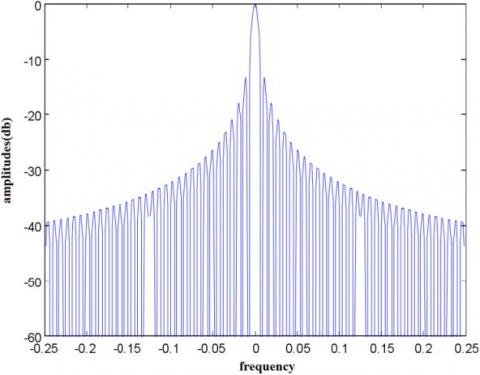
The FFT was introduced to complete the MTD and coherent accumulation for signal processing of traveling detection pulse radar (Cooley et al., 1988). To realize the MTD by FFT algorithm, the received samples $\mathrm{S}=\lceil S[1] S[2] \cdots S[m]\rceil^{T}$ can be processed as:
$\widehat{\Phi}_{F F T}(f)=\frac{1}{M}\left|\sum_{m=1}^{M} s[m] e^{-j 2 \pi m f}\right|^{2}$ (7)
Suppose there are m = 128 in a processing period. Then, the spectrum of a single filter is shown in Figure 5.
Figure 5. Amplitude-frequency features of FFT Filters
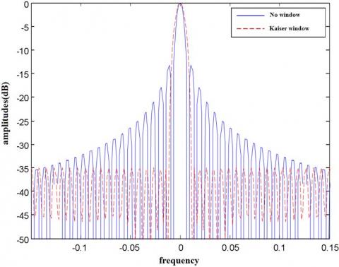
As shown in Figure 5, the MTD and coherent accumulation can be completed if the FFT is processed directly from time-domain data, and the sidelobe is -13.2dB. The FFT filter bank should be windowed to reduce the sidelobe level. The commonly used window functions include Kaiser window, Chebyshev window, Hamming window and Hanning window. Each of these window functions has its advantages.
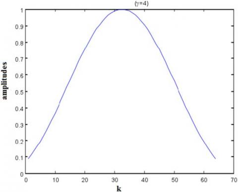
Taking the Kaiser window for example, when the width of the main lobe is equal to that of the corresponding fixed window, the lower sidelobe can be obtained by choosing parameter $\gamma$, or the narrower main lobe can be obtained under the given sidelobe condition. When $\gamma$=4, the time-domain and frequency-domain features of Kaiser window function are shown in Figure 6 and Figure 7, respectively.
Figure 6. Time-domain of Kaiser window function ($\gamma$=4)
Figure 7. Frequency-domain of Kaiser window function ($\gamma$=4)
The windowed FFT of the received signals s can be calculated as:
$\widehat{\emptyset}_{F F T W}(f)=\frac{1}{M P}\left|\sum_{m=1}^{M} w[m] S[m] e^{-j 2 \pi m f}\right|^{2}$ (8)
where P is the power of the time window $\{w[m]\}$
.$P=\frac{1}{M} \sum_{m=1}^{M} w[m]^{2}$ (9)
Figure 8 compares the spectra of FFT filters with and without window.
Figure 8. Spectrum comparison between FFT filters with and without window
5.1. Construction of 3D geographic scene
The 3D geographic scene provides accurate inputs of location information, while the information of the radar, the jamming source and the target were configured in advance according to the scene.
The maximum detection range of the radar depends on the maximum operating range. Here, the latter is defined by a classical radar equation, in which the detection range of the radar $R_{\text {max }}$ reaches the maximum when the power $P_{r}$ of the target echo signal received by the radar equals the smallest detectable power $S_{\text {min }}$ of the radar receiver:
$R_{\max }=\left[\frac{P_{t} G_{t} G_{r} \lambda^{2} \sigma}{(4 \pi)^{3} S_{\min }}\right]^{\frac{1}{4}}$ (10)
where $R_{\max }$ is the maximum detection range of the radar; $P_{t}$ is the peak power of the radar transmitter; $G_{t}$ and $G_{r}$ are the gains of the radar transmitter and radar receiver, respectively; $\lambda$ is the working wavelength of the radar; $\sigma$ is the target effective reflection area; $S_{\min }$ is the smallest detectable power of the radar receiver, i.e. the radar sensitivity.
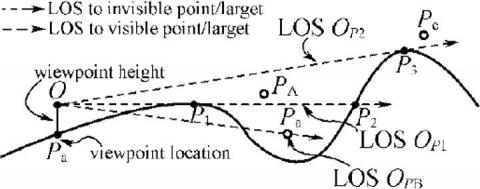
The terrain shading factor should be considered before displaying the 3D detection range of the radar in a 3D geographic scene. In this paper, the terrain model is described by a digital elevation model with regular grid spacing. The 2.5D topographic surface was divided continuously into several 1.5D topographic curves. The visual field of the viewpoint (O) was determined by traversing and judging the visibility of the sampling points on each topographic curve. The profile is radial distribution centered on viewpoint O. A section of the shaded area is shown in Figure 9, where L is the section curve.
Figure 9. A section of the shaded area
In this way, the problem is transformed into how to determine the visibility of the sampling point on a 2D curve to the viewpoint O (Figure 10).
Figure 10. Corresponding 2D curve
The lowest visible height at each location could be obtained by the traveling detection pulse radar. All the calculated data on the visibility at the boundary points of radar detection range were stored in a 2D matrix, and then rendered and displayed on a 3D geographic information system (GIS) platform. In this way, a 3D radar detection range model was obtained. To calculate the 2D detection range at a specified height, the detection range at that height was obtained by retrieving the data from the 2D matrix corresponding to that height, and rendering the data for display. Figure 11 shows a 3D geographic scene of detection range generated through signal processing of traveling detection pulse radar.
Figure 11. 3D geographic scene of detection range generated through signal processing of traveling detection pulse radar
5.2. Experimental verification
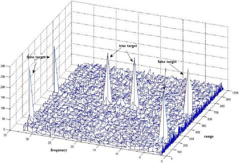
The proposed method can correct the target Doppler channel value according to the attitude sensor and servo azimuth data. To verify the accuracy of the proposed method, the radar is placed in the normal traveling detection mode, and the target position was determined with and without speed compensation. Figure 12 and Figure 13 respectively show the 3D target detected without and with speed compensation.
Figure 12. Target detected without speed compensation
Figure 13. Target detected with speed compensation
The comparison shows that the false targets caused by radar motion were successfully eliminated by speed compensation. This means the proposed method is feasible for application.
Firstly, the principle and basic methods of target detection and signal processing of pulse radar signal processing were reviewed, and the typical algorithms of signal processing were introduced in details. Then, the problem and solutions of traveling radar detection were discussed, and the principle and realization means of each compensation algorithm were analyzed in turns. On this basis, the author realized the travelling radar detection of moving target and created a 3D model for the detection process based on 3D geographic scene. The experimental results show that the 3D geographic scene is realistic and accurate, and the proposed method is feasible for application.
Antipov I., Baldwinson J. (2008). Estimation of a constant false alarm rate processing loss for a high-resolution maritime radar system. Journal of Physiology, Vol. 570, No. 2, pp. 295-307. http://dx.doi.org/10.1113/jphysiol.2005.097378
Becker A. (1987). Integrated navigation, communication and surveillance systems based on standard distance measuring equipment. Journal of Navigation, Vol. 40, No. 2, pp. 194-205. http://dx.doi.org/10.1017/S0373463300000448
Cooley J. W., Lewis P. A. W., Welch P. D. (1988). The fast fourier transform and its applications. Education IEEE Transactions on, Vol. 12, No. 1, pp. 27-34. http://dx.doi.org/10.1109/te.1969.4320436
Du D., Li K., Fei M. (2010). A fast multi-output RBF neural network construction method. Neurocomputing, Vol. 73, No. 10, pp. 2196-2202. http://dx.doi.org/10.1016/j.neucom.2010.01.014
Fan B., Wang J., Qin Y., Wang H., Xiao H. (2014). Polar format algorithm based on fast gaussian grid non-uniform fast fourier transform for spotlight synthetic aperture radar imaging. Radar Sonar & Navigation Iet, Vol. 8, No. 5, pp. 513-524. http://dx.doi.org/10.1049/iet-rsn.2013.0199
Guo Q., Qu Z., Wang C. (2010). Pulse-to-pulse periodic signal sorting features and feature extraction in radar emitter pulse sequences. Journal of Systems Engineering & Electronics, Vol. 21, No. 3, pp. 382-389. http://dx.doi.org/10.3969/j.issn.1004-4132.2010.03.006
He A. L., Zeng D. G., Wang J., Tang B. (2009). Multi-parameter signal sorting algorithm based on dynamic distance clustering. Journal of Electronic Science and Technology, Vol. 7, No. 3, pp. 249-253.
Klilou A., Belkouch S., Elleaume P., Le Gall P., Bourzeix F., Hassani M. (2014). Real-time parallel implementation of pulse-doppler radar signal processing chain on a massively parallel machine based on multi-core DSP and serial RAPIDIO interconnect. EURASIP Journal on Advances in Signal Processing, Vol. 2014, No. 1, pp. 161. http://dx.doi.org/10.1186/1687-6180-2014-161
Liu B., Shi P. (2009). Delay-range-dependent stability for fuzzy bam neural networks with time-varying delays. Physics Letters A, Vol. 373, No. 21, pp. 1830-1838. http://dx.doi.org/10.1016/j.physleta.2009.03.044
Malvezzi M., Allotta B., Rinchi M. (2011). Odometric estimation for automatic train protection and control systems. Vehicle System Dynamics, Vol. 49, No. 5, pp. 723-739. http://dx.doi.org/10.1080/00423111003721291
Meng D., Feng Z., Mingquan L. U. (2008). Anti-jamming with adaptive arrays utilizing power inversion algorithm. Tsinghua Science & Technology, Vol. 13, No. 6, pp. 796-799. http://dx.doi.org/10.1016/S1007-0214(08)72202-8
Montazer G. A., Khoshniat H., Fathi V. (2013). Improvement of RBF neural networks using fuzzy-osd algorithm in an online radar pulse classification system. Applied Soft Computing Journal, Vol. 13, No. 9, pp. 3831-3838. http://dx.doi.org/10.1016/j.asoc.2013.04.021
Rui Z., Yi M. S., Peng Z. Y., Lin L. X. (2002). Implementation of the secondary surveillance radar signal processor based on DSP-FPGA. Systems Engineering & Electronics, Vol. 24, No. 12, pp. 8-11. http://dx.doi.org/10.1002/mop.10502
Wang S. J., Si X. C. (2003). Research on an improved sorting method for radar signal. Systems Engineering & Electronics, Vol. 25, No. 9, pp. 1079-1083. http://dx.doi.org/10.3321/j.issn:1001-506X.2003.09.011
Wang S. Q. (2011). Multi-parameter radar signal sorting method based on fast support vector clustering and similitude entropy. Journal of Electronics & Information Technology, Vol. 33, No. 11, pp. 2735-2741. http://dx.doi.org/10.3724/SP.J.1146.2011.00261
Xiao W. H., Wu H. C., Yang C. Z., Wang M. L. (2013). An improved sdif radar pulse signal main sorting algorithm. Advanced Materials Research, Vol. 710, pp. 637-641. http://dx.doi.org/10.4028/www.scientific.net/AMR.710.637