Suat Toraman
© 2020 IIETA. This article is published by IIETA and is licensed under the CC BY 4.0 license (http://creativecommons.org/licenses/by/4.0/).
OPEN ACCESS
Epilepsy is a neurological disease affecting almost 1% of world population. Predicting a possible seizure will make a significant contribution to improving the quality of life of patients suffering from this disease. One of the most important steps in seizure prediction studies is the preictal activity recognition stage. In many previous studies, the preictal state was determined to end at the onset of the seizure, which makes it difficult for the physician to intervene in the patient in a possible seizure. In the proposed method, unlike previous studies, the preictal state was determined as the 30-minute interval ending 30 minutes before the onset of an epileptic seizure. The method consisted of three stages; (I) preictal and interictal activities were divided into five-second segments, (ii) the separated signals were converted into spectrograms, and (iii) the spectrogram images were classified using three different pre-trained CNN models (VGG19, ResNet, DenseNet) and the results were compared among these models. Classification was performed separately using the predetermined four EEG channels for 20 cases in the CHB-MIT dataset. The best classification accuracy value in preictal/interictal discrimination (91.05%) was obtained on channel 8 (P3-O1). An important contribution of this study was that the proposed approach provided important information about the preictal and interictal discrimination of the section 30 minutes before the onset of seizures. In addition, by examining the four channels separately, channel-based information on preictal/interictal discrimination was also obtained. Based on these results, we consider that the proposed method will bring a different perspective to seizure prediction studies.
biomedical image processing, EEG, epilepsy, preictal, convolutional neural network, deep learning
Epilepsy is a neurological disease of the central nervous system (CNS), affecting approximately 1% of the world population [1]. The disease occurs by unpredictable seizures due to sudden malfunction during normal activities of neurons [1, 2]. An electroencephalogram (EEG) testing is used to examine changes in the electrical brain activity causing epilepsy and to identify any seizure that may occur. The important point in seizure prediction is to determine the preictal state in which the changes in brain activity begin to occur. With a strong seizure prediction system, the disease can be controlled easily [2]. Before the seizure begins, taking the necessary precautions can easily predict and even prevent the seizure. Therefore, it is highly important to determine the preictal state that contains important information for a seizure prediction.
Recently, researchers have used various methods to detect changes in brain activity. These methods can be divided into two groups: (I) features extracted manually from the EEG signals and classified with various classifiers (neural network, support vector machines (SVM), multi-layer perceptron, and linear discriminant analysis) and (II) automatic feature extraction and classification that are carried out with deep learning methods. Studies reporting on both methods are examined below.
Zhou et al. performed a seizure detection system using Lacunarity and Bayesian linear separation analysis [3]. Rana et al. used the phase-slope index (PSI) of EEG signals to determine epileptic seizures from the frequency domain [4]. Liu et al. divided the multichannel intracranial EEG signals into its sub-bands by the wavelet transform and classified them by extracting various features [5]. Tafreshi et al. examined the performance of the Empirical Mode Decomposition to distinguish between normal and epileptic seizure data [6]. Zhang et al. used the spectral analysis of scalp EEG signals to distinguish between preictal and interictal EEG segments [7]. Cho et al. used phase-locking values to classify EEG signals as interictal or preictal [8]. Tsiouris et al. classified preictal and interictal states using the features obtained by the frequency domain, time domain, and graph theory [2]. Subaşı et al. divided EEG signals into sub-bands by wavelet transform, whereby the features were extracted by PCA, LDA, and IDA and were classified accordingly [9]. In all these methods, feature extraction was performed using EEG signals by various signal processing techniques and these features were classified accordingly [10, 11].
Additionally, given that seizure characteristics differ among patients, distinguishing distinctive features from EEG signals is highly important. In recent years, deep learning methods that have gained popularity with AlexNet play an important role in this issue. Deep learning models allow automatic feature identification without requiring hand-crafted feature extraction and selection from raw data. Deep learning has become a highly preferred method in medical sciences due to its successful results in signal/image processing and classification [12, 13]. Automatic feature extraction by deep learning provides better outcomes than traditional methods such as hand-crafted feature extraction [14]. Recently, applications used for examining EEG signals have also become popular due to an increasing interest in deep learning methods [15, 16]. Among these, there are various applications analyzing EEG signals in the form of one-dimensional signals or two-dimensional images. Yıldırım et al. classified EEG signals as normal and abnormal [17] using a 1D convolutional neural network (CNN) model. Toraman et al. converted EEG signals to 2-D spectrogram images and classified them after the feature extraction to determine the laterality of speech [18]. Ullah et al. automatically classified EEG signals as normal, ictal, and interictal [19]. Fahimi et al. suggested a CNN-based method for the detection of mental state from single-channel raw EEG data [20]. Supratak et al. proposed a deep learning model called DeepSleepNet for automatic sleep stage scoring [21]. Oh et al. proposed a CNN model using EEG signals for automatic detection of Parkinson’s disease [22].
1.1 Motivation and contribution
Epilepsy is a disease negatively affecting patients’ daily life and reducing their quality of life. For this reason, various machine learning methods have been developed to assist physicians in the decision-making processes regarding the detection of epilepsy. In this study, a method for determining preictal/interictal activities, which are one of the most important steps in seizure prediction, is proposed. In the proposed method, three pre-trained CNN models (VGG19, ResNet, DenseNet) were used to recognize preictal EEG signals. The CNN models were trained by converting one-dimensional EEG signals to 2D spectrogram images and were classified. The contributions of this paper could be summarized as follows:
- To the best of our knowledge, this is the first study to extract and classify the properties of spectrogram images obtained from preictal and interictal signals using the transfer learning approach.
- Data were classified as preictal and interictal without requiring any hand-crafted feature extraction technique.
- One-dimensional scalp EGG signals were transformed to 2D spectrogram images with an in-depth learning approach and were trained by pre-trained CNN models.
- The transfer learning approach eliminates the challenges such as determination of hyperparameters in the training and design stage of the model.
- A channel-based examination was performed to determine the preictal time, which is vitally important for seizure prediction.
- In addition, unlike other studies, the preictal period was determined as the period that ended 30 minutes before the onset of seizures. Moreover, the effectiveness of this stage for predicting a seizure was also demonstrated in the study.
The rest of the study is organized as follows: Chapter 2 provides fundamental information on the selection of preictal/interictal activities, CNN models, performance evaluation criteria, and data sets, Chapter 3 contains the experimental results, Chapter 4 presents the discussion of findings, and Section 5 presents the conclusion of the study.
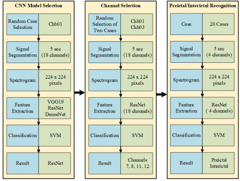
In this study, a deep learning method for preictal/interictal recognition, which is an important step in seizure prediction applications, is proposed. Feature extraction was employed for differentiating the preictal and interictal states from scalp EEG signals using trained CNN models with millions of images. EEG signals were converted to spectrogram images and were used as input data to 2D CNN models. The preictal/interictal differentiation was performed using the extracted features. The flow diagram of the study is given in Figure 1.
Figure 1. Flow diagram of the proposed method
Figure 2. 18-channel samples and the electrode positions placed according to the 10-20 system during EEG recordings
2.1 EEG dataset
In this study, the publicly available CHB-MIT scalp EEG dataset was used [23]. EEG signals were collected from children who were receiving treatment for seizures in Boston Children’s Hospital. All EEG signals were obtained from 18 to 23 channels and were sampled at 256 Hz. Figure 2 shows the 10-20 System of EEG Electrode Placement used for collecting EEG signals.
Total duration of the EEG recordings was 983 hours. Most EEG recordings consisted of 1-h epochs, while others were 2 to 4-h epochs. The seizure onset and offset times were marked by a clinical expert. In the annotation file of the data set, channel changes, seizure start/end information was given. Table 1 shows the information for the CHB-MIT EEG data set.
Table 1. CHB-MIT EEG data set description
|
Case |
Gender |
Age (years) |
# of seizure |
Length (hh: mm: ss) |
number of seizures used |
|
chb01 |
F |
11 |
7 |
40:33:08 |
5 |
|
chb02 |
M |
11 |
3 |
35:15:59 |
2 |
|
chb03 |
F |
14 |
7 |
38:00:06 |
2 |
|
chb04 |
M |
22 |
4 |
156:03:54 |
3 |
|
chb05 |
F |
7 |
5 |
39:00:10 |
4 |
|
chb06 |
F |
1,5 |
10 |
66:44:06 |
7 |
|
chb07 |
F |
14,5 |
3 |
67:30:08 |
3 |
|
chb08 |
M |
3,5 |
5 |
20:00:23 |
4 |
|
chb09 |
F |
10 |
4 |
67:52:18 |
3 |
|
chb10 |
M |
3 |
7 |
50:01:24 |
4 |
|
chb11 |
F |
12 |
3 |
34:47:37 |
- |
|
chb12 |
F |
2 |
40 |
20:41:40 |
- |
|
chb13 |
F |
3 |
12 |
33:00:00 |
3 |
|
chb14 |
F |
9 |
8 |
26:00:00 |
3 |
|
chb15 |
M |
16 |
20 |
40:00:36 |
9 |
|
chb16 |
F |
7 |
10 |
19:00:00 |
3 |
|
chb17 |
F |
12 |
3 |
21:00:24 |
1 |
|
chb18 |
F |
18 |
6 |
35:38:05 |
2 |
|
chb19 |
F |
19 |
3 |
29:55:46 |
- |
|
chb20 |
F |
6 |
8 |
27:36:06 |
2 |
|
chb21 |
F |
13 |
4 |
32:49:49 |
2 |
|
chb22 |
F |
9 |
3 |
31:00:11 |
2 |
|
chb23 |
F |
6 |
7 |
26:33:30 |
4 |
For this study, the preictal interval was determined as the 30-minute interval ending 30 minutes before the seizure onset. This duration was determined since it is highly important to give an effective time for the physician to intervene in the patient before the seizure onset [16]. Moreover, the preictal interval is an arbitrary choice of investigators since there is no precise time limit for the preictal state [2]. Therefore, in this study, the preictal window of 30 min was chosen. The 10-min time period after the seizure was determined as the postictal state [24]. There were various seizures that occurred over a short interval in the CHB-MIT EEG data set, of which the seizure that occurred first was included in the analysis There were 20 cases that fulfilled the inclusion criteria (see Table 1). The time periods other than the preictal, ictal, and postictal periods were accepted as interictal, which occurred at least two hours away from the seizure [2]. In addition, segments were chosen as non-overlapping 5 sec as in the study [2]. Figure 3 shows an example of a signal for the identification of preictal and interictal periods.
Figure 3. Brain activities of epilepsy patients include interictal, preictal, ictal, and postictal states. The first 30-min period before each seizure was defined as the preictal period
2.2 Preictal state detection
The preictal detection approach consisted of the segmentation of EEG signals, conversion of each segment into spectrogram, extraction of deep features from spectrogram images, and the classification stages (Figure 1).
2.2.1 Segmentation
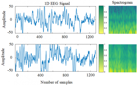
For one patient who had a history of five seizures, a 150-min (5x30) preictal state and a 150-min interictal state were randomly selected. The time periods defined as ictal in the annotation file were not used. The EEG signals were then segmented for each case in the data set. Figure 4 shows some examples of preictal and interictal signals that were divided into 5-sec segments. The sliding window method was used for segmentation, which can be used with or without overlap. The overlapping sliding window analysis is highly useful for data continuity although it causes redundant information. The analysis of 18-channel data of each patient resulted in excessive information density, which can cause serious problems both in terms of processing load and timing. Accordingly, the EEG signals were divided into non-overlapping segments.
2.2.2 Spectrogram
Since a 2D CNN model was used in the study, the segmented raw EEG signals were converted to 2D image format. Methods such as Short-time Fourier Transform (STFT) and Wavelet transform were used effectively in image conversion and feature extraction since these methods retain the time-frequency information in the analysis of signals [25]. All preictal and interictal activities were divided into 5-sec segments. While obtaining the spectrogram, the hamming window width was selected as 16 ms, overlap 8 ms, and 512-point Fast Fourier Transform (FFT) was used. The Viridis scales were employed to provide a color map. Figure 4 shows the spectrograms examples of preictal and interictal segments. The obtained spectrogram images were of 875 x 656 pixels. The pre-trained VGG19, ResNet and DesNet models have an original input size of 224 x 224 pixels. Additionally, using large images for input requires more hardware resources and increases processing load. Therefore, each spectrogram image was resized to 224 x 224 pixels.
Figure 4. 5-sec segmented preictal/interictal EEG signals
2.2.3 CNN
CNN models have been shown to provide successful results in classification and detection in medical applications [14, 26]. These models became more popular with the success in the ImageNet Large Scale Visual Recognition Challenge (ILSVRC) in 2012 by Krizhevsky et al. [27]. Moreover, the advent of VGGNet and ResNet further increased this popularity in 2014 and in 2015, respectively. A good training process is needed for a CNN model to achieve a good classification or recognition. Additionally, a large amount of data is required for good training, which mostly cannot be obtained. In such cases, using pre-trained models with large data sets produces more successful results. Instead of re-training a CNN model, it is easier to perform a process using the weights of pre-trained models. This method is called Transfer Learning, which allows a more efficient feature extraction from smaller data sets and also allows the training of small data sets with low computation costs [28]. In this study, VGG19, ResNet, and DenseNet models were used to extract deep features. For each spectrogram image, VGG19, ResNet, and DenseNet produced feature vectors of length 4096, 2048, and 1920, respectively.
VGG19: CNN models, which began with LeNet and then become popular with AlexNet, were effectively used by the Visual Geometry Group of Oxford University (VGG) in the development of VGG16. VGG16 consists of 13 convulsion layers and 3 fully connected layers and VGG19 consists of 16 convulsion layers and 3 fully connected layers. There are also 5 max-pooling and softmax layers which are the final layers in both models. While softmax is used to classify data, ReLu is used as the activation function [19, 29, 30].
ResNet: The earliest CNN models had a remarkably low number of layers. Of note, VGG16 had 8 layers and VGG19 had 16 layers. However, with the rapid developments in GPU technology, the number of layers in CNN models increased. One of these models is ResNet architecture, in which different architectural structures with 50, 101, and 152 layers have been used. In deep CNN architectures, the number of layers was increased, which made the training difficult. As a result, the input and gradient values started to vanish. In order to solve this problem, the skip connection technique was used in ResNet, whereby the output of one layer was added to the next input by skipping certain layers and thus a more effective training model was provided [31, 32].
DenseNet: DenseNet has a structure in which the previous layer properties are forwarded to all subsequent layers. Unlike ResNet, DenseNet transfers the previous layer information to all subsequent layers, instead of skipping some layers and transferring the previous layer information to the next layers. This provides a stronger flow of information between the layers. Another advantage of DenseNet is that it creates inputs by adding information from the previous layer to the next layer, rather than collecting features when creating layer inputs [33].
2.2.4 Support Vector Machine
Support Vector Machine (SVM) is a machine learning algorithm used for separating data sets with two or more classes by finding an optimal hyperplane. SVM reduces structural risks and uses support vectors to separate classes. After determining support vectors, the most appropriate hyperplane to separate the data set is found. In the two-class data set $\left\{x_{i}, y_{i}\right\} i=1,2,3,4, \ldots, k, y_{i} \in\{-1,+1\}$ are the class labels in the dataset [34, 35]. Inequalities that define the most appropriate hyperplane to separate classes are described as follows:
$\begin{array}{cl}w \cdot x_{i}+b \leq 1, & y=-1 \\ w. x_{i}+b \geq 1, & y=1\end{array}$ (1)
As a result, the obtained separation function for the two-class data set that can be separated linearly is as follows:
$f(x)=\operatorname{sign}\left(\sum_{i=1}^{k} \alpha_{i} y_{i} K\left(x. x_{i}\right)+b\right)$ (2)
Here, α represents the Lagrange multiplier, b represents bias, $x_{i}$ represents support vectors and K represents kernel functions [34, 35]. The Kernel functions used in the study included Radial Basis Function (RBF), Polynomial, and Linear.
2.2.5 Performance evaluation
The k-fold cross-validation method was used to evaluate the performance of the proposed method. The k value was determined as 5 and thus the data set was divided into 5 parts. Four parts were used for training and the remaining part was used for testing. This procedure was applied to all parts. The average of five values was calculated for performance evaluation. The parameters used for performance comparison were defined as True Positive (TP), which represented the number of precisely defined preictal segments, as False Negative (FN), which represented the number of incorrectly defined preictal segments, as True Negative (TN), which represented the number of correctly defined interictal segments, and as False Positive (FP), which represented the number of incorrectly defined interictal segments.
Sensitivity $=\mathrm{TP} /(\mathrm{TP}+\mathrm{FN}) \times 100$ (3)
Specificity $=\mathrm{TN} /(\mathrm{TN}+\mathrm{FP}) \times 100$ (4)
Accuracy $=(\mathrm{TP}+\mathrm{TN}) /(\mathrm{TP}+\mathrm{FP}+\mathrm{TN}+\mathrm{FN}) \times 100$ (5)
In the proposed model, EEG signals were transformed into a spectrogram image using MATLAB software. Other applications were implemented using the KERAS 2.1.6 library in Python 3.5. Training and testing of the model were performed on a Linux server with NVIDIA GTX 1080 graphics card.
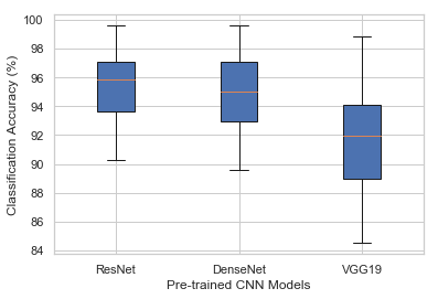
In this study, a two-stage method was used to analyze preictal and interictal activities. In the first stage, feature extraction was performed with three pre-trained deep learning architectures using a random case, and the extracted features were classified with SVM. Based on the classification results, it was determined as to which CNN architecture was more successful in differentiating preictal and interictal activities. The case selected for classification was chb01 and there were five seizures in the chb01 case that were appropriate for the study conditions. Five seizures from chb01 were examined with three different CNN models. A 30-min preictal section was selected for each seizure. For five seizures, a 150-min (5 x 30) preictal state and a 150-min interictal state were randomly selected. The interictal state was determined as the time period at least two hours away from the onset and the end of the seizure. The 150-min preictal and interictal activities were divided into 1800 segments with a 5-s non-overlapping sliding window. A total of 3600 spectrogram images were obtained by converting each segment into a spectrogram image. Feature vectors were obtained from spectrogram images using VGG19, ResNet, and DenseNet. Feature vectors were classified as preictal and interictal by SVM using 5-fold cross-validation. The classification results for 18 channels of the chb01 case are shown in Table 2.
As shown in Table 2, ResNet achieved the best result in 13 out of 18 channels, while DenseNet achieved higher values in 5 channels. The VGG19, however, did not achieve a higher success in any channel when compared to the other two CNN models, which could be due to the fact that VGG19 has a shallower architecture than those of ResNet and DenseNet. Based on these results, ResNet was chosen as the CNN model to be used in the study. In Figure 5, the accuracy of the three CNN models is compared.
After determining the CNN model to be used in the first stage, the channels to be used in the second stage were determined. Considering that more hardware resources and time were needed to examine all the channels, the number of channels to be examined was determined as four. In order to decide which four channels out of 18 channels to use, the ResNet results of 18 channels were compared for two cases, chb01 and chb03, which were randomly selected. Table 3 presents the ResNet accuracy results for two cases.
Table 2. 18-channel classification accuracy of the chb01 case with ResNet, DenseNet, and VGG19
|
Channels |
ResNet |
DenseNet |
VGG19 |
|
Channel 1 |
93.83 ± 3.26 |
93.14 ± 2.95 |
88.58 ± 3.12 |
|
Channel 2 |
90.83 ± 1.76 |
91.03 ± 2.81 |
84.50 ± 2.27 |
|
Channel 3 |
90.31 ± 1.59 |
89.56 ± 1.77 |
88.14 ± 1.81 |
|
Channel 4 |
94.69 ± 1.23 |
94.39 ± 1.95 |
91.00 ± 1.33 |
|
Channel 5 |
93.58 ± 1.64 |
92.92 ± 2.33 |
90.92 ± 2.60 |
|
Channel 6 |
96.92 ± 0.97 |
95.64 ± 0.80 |
93.44 ± 1.26 |
|
Channel 7 |
99.64 ± 0.42 |
99.58 ± 0.46 |
98.56 ± 1.32 |
|
Channel 8 |
99.58 ± 0.00 |
99.61 ± 0.21 |
98.89 ± 0.70 |
|
Channel 9 |
95.83 ± 1.47 |
94.89 ± 1.46 |
93.42 ± 1.43 |
|
Channel 10 |
94.69 ± 0.98 |
93.42 ± 1.91 |
92.11 ± 1.59 |
|
Channel 11 |
98.86 ± 0.73 |
98.92 ± 0.71 |
97.11 ± 1.44 |
|
Channel 12 |
98.58 ± 0.92 |
98.78 ± 0.85 |
96.25 ± 0.82 |
|
Channel 13 |
96.78 ± 0.41 |
97.31 ± 1.27 |
91.83 ± 2.16 |
|
Channel 14 |
92.22 ± 1.20 |
92.08 ± 2.06 |
84.75 ± 2.04 |
|
Channel 15 |
92.22 ± 2.20 |
91.06 ± 2.78 |
87.31 ± 2.53 |
|
Channel 16 |
97.14 ± 0.69 |
96.47 ± 1.42 |
94.33 ± 1.55 |
|
Channel 17 |
95.92 ± 1.22 |
95.14 ± 0.70 |
92.92 ± 1.83 |
|
Channel 18 |
96.00 ± 1.44 |
95.89 ± 1.32 |
90.14 ± 2.19 |
|
Mean ± SD |
95.42 ± 1.22 |
94.99 ± 1.54 |
91.90 ± 1.77 |
Table 3. Classification accuracy of 18 channels with ResNet for cases chb01 and chb03
|
Channels |
chb01 |
chb03 |
|
Channel 1 |
93.83 ± 3.26 |
87.78 ± 2.89 |
|
Channel 2 |
90.83 ± 1.76 |
83.75 ± 3.33 |
|
Channel 3 |
90.31 ± 1.59 |
87.92 ± 2.08 |
|
Channel 4 |
94.69 ± 1.23 |
92.36 ± 2.11 |
|
Channel 5 |
93.58 ± 1.64 |
85.69 ± 2.76 |
|
Channel 6 |
96.92 ± 0.97 |
85.00 ± 5.56 |
|
Channel 7 |
99.64 ± 0.42 |
97.36 ± 2.62 |
|
Channel 8 |
99.58 ± 0.00 |
98.54 ± 0.28 |
|
Channel 9 |
95.83 ± 1.47 |
89.24 ± 2.45 |
|
Channel 10 |
94.69 ± 0.98 |
89.17 ± 3.96 |
|
Channel 11 |
98.86 ± 0.73 |
98.12 ± 1.94 |
|
Channel 12 |
98.58 ± 0.92 |
97.78 ± 0.83 |
|
Channel 13 |
96.78 ± 0.41 |
85.83 ± 2.96 |
|
Channel 14 |
92.22 ± 1.20 |
81.87 ± 5.78 |
|
Channel 15 |
92.22 ± 2.20 |
87.15 ± 3.20 |
|
Channel 16 |
97.14 ± 0.69 |
93.82 ± 3.44 |
|
Channel 17 |
95.92 ± 1.22 |
98.54 ± 1.42 |
|
Channel 18 |
96.00 ± 1.44 |
99.24 ± 0.81 |
|
Mean ± SD |
95.42 ± 1.22 |
91.06 ± 2.69 |
Figure 5. Boxplot of classification accuracy obtained by ResNet, DenseNet, and VGG19 using 18 channels for the chb01 case
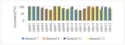
As shown in Table 3, the highest accuracy values for the chb01 case were obtained in channel 7, 8, 11, and 12, while the highest accuracy values for the chb03 case were obtained in channel 8, 11, 12, and 18. Some of the cases were not included in the comparison because there was no continuity in channel 5, 10, 13, and 18. Therefore, in the chb03 case, the best four channels were identified as 8, 11, 12, and 17. In the Chb01 and chb03 cases, channel 8, 11, and 12 had the highest values. However, whether to use ch7 or ch17 for the chb03 case was determined based on the average values of ch7 and ch17 for chb01 and chb03. The ch7 was chosen as the 4th channel since its average value was the highest. Figure 6 illustrates the comparison of the accuracy values obtained for chb01 and chb03.
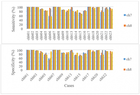
After the comparison of channels for chb01 and chb03, the classification accuracy of the other cases was calculated for the four channels chosen. The classification accuracy of all cases is presented in Table 4. The highest mean accuracy value was obtained for channel 8 (91.05%), while the lowest accuracy was achieved for channel 7 (88.71%). The mean classification accuracy value of the four channels for 20 cases was found as around 90%. The mean classification performance of 10 cases for four channels was above 90%, while the average of 3 cases was below 80%. Epilepsy has a structure that varies from person to person, from seizure to seizure [36]. This notion was confirmed by our findings that indicated that the accuracy values of the examined EEG channels were high in some patients and were low in the other patients. As a matter of fact, this variability makes the development of a general seizure prediction system very difficult. On the other hand, it was also revealed that the 30-min interval determined as the preictal period contained important information for the preictal and interictal distinction. The classification accuracy of 20 cases for four channels is comparatively given in Figure 7. Figure 8 illustrates the sensitivity and specificity values of 20 cases for four channels.
Table 4. The accuracy values of 20 cases in four channels
|
Case |
Channel 7 |
Channel 8 |
Channel 11 |
Channel 12 |
|
chb01 |
99.64 ± 0.42 |
99.58 ± 0.00 |
98.86 ± 0.73 |
98.58 ± 0.92 |
|
chb02 |
99.38 ± 1.19 |
99.51 ± 0.56 |
99.31 ± 0.76 |
99.44 ± 1.13 |
|
chb03 |
97.36 ± 2.62 |
98.54 ± 0.28 |
98.12 ± 1.94 |
97.78 ± 0.83 |
|
chb04 |
86.90 ± 2.49 |
92.22 ± 1.42 |
91.62 ± 3.43 |
88.89 ± 4.32 |
|
chb05 |
78.85 ± 2.46 |
82.19 ± 3.32 |
82.81 ± 2.61 |
79.48 ± 1.93 |
|
chb06 |
74.88 ± 2.19 |
72.87 ± 1.87 |
74.66 ± 1.65 |
74.38 ± 1.56 |
|
chb07 |
100.00 ±0.00 |
100.00 ±0.00 |
99.95 ± 0.19 |
100.00 ±0.00 |
|
chb08 |
99.20 ± 0.64 |
99.17 ± 0.51 |
99.13 ± 1.18 |
99.44 ± 0.40 |
|
chb09 |
86.32 ± 1.57 |
85.21 ± 1.48 |
87.85 ± 2.83 |
85.49 ± 2.61 |
|
chb10 |
77.33 ± 2.03 |
85.73 ± 2.28 |
79.86 ± 3.20 |
89.31 ± 2.48 |
|
chb13 |
91.90 ± 1.63 |
99.12 ± 0.80 |
98.29 ± 0.37 |
83.98 ± 2.90 |
|
chb14 |
75.69 ± 0.29 |
77.59 ± 4.77 |
73.52 ± 2.82 |
85.60 ± 2.96 |
|
chb15 |
71.96 ± 1.22 |
74.61 ± 1.55 |
70.42 ± 2.66 |
70.05 ± 1.41 |
|
chb16 |
84.12 ± 3.33 |
82.18 ± 2.50 |
84.49 ± 1.94 |
80.69 ± 3.89 |
|
chb17 |
99.17 ± 1.04 |
99.86 ± 0.56 |
99.72 ± 1.11 |
100.00 ±0.00 |
|
chb18 |
93.96 ± 1.62 |
98.33 ± 1.19 |
90.14 ± 3.53 |
94.24 ± 2.35 |
|
chb20 |
98.54 ± 1.02 |
98.82 ± 1.13 |
98.47 ± 0.34 |
99.17 ± 0.34 |
|
chb21 |
75.14 ± 3.69 |
85.14 ± 2.17 |
99.24 ± 0.52 |
76.94 ± 3.25 |
|
chb22 |
95.42 ± 2.21 |
95.90 ± 1.83 |
95.28 ± 1.50 |
91.11 ± 1.99 |
|
chb23 |
88.51 ± 1.60 |
94.37 ± 0.97 |
81.77 ± 2.80 |
91.32 ± 1.24 |
|
Mean±SD |
88.71 ± 1.66 |
91.05 ± 1.46 |
90.17 ± 1.80 |
89.29 ± 1.82 |
Figure 6. Classification accuracy of 18 channels for chb01 and chb03
Figure 7. Graphical comparison of the accuracy values of 20 cases for the selected four channels
Figure 8. Sensitivity (top) and specificity (bottom) of 20 cases for four channels
Figure 9. ROC Curves of the classification accuracy of six cases for Channel 8. a) chb01, b) chb02, c) chb03, d) chb04
Table 5. The accuracy, sensitivity, and specificity values of 20 cases
|
Parameter |
Channel 7 |
Channel 8 |
Channel 11 |
Channel 12 |
|
Acc |
88.71 |
91.05 |
90.17 |
89.29 |
|
Sen |
88.59 |
92.31 |
90.97 |
88.28 |
|
Spe |
87.54 |
89.76 |
89.37 |
90.25 |
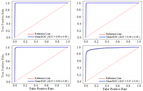
Table 5 shows the average accuracy, sensitivity, and specificity values of 20 cases for four channels. The receiver operating characteristic (ROC) curve is commonly used in machine learning applications for measuring the performance of a model. The area under the ROC curve (AUC) is a numerical measure of the model’s ability to separate the dataset. In the ROC curve analysis, the closer the ROC curve is to the upper left corner, the higher the overall accuracy of the test in separating data sets. Figure 9 shows the ROC curves of the classification accuracy of 20 cases in channel 8. In ROC graphs, the thick blue curve represents the average ROC curve obtained by 5-fold cross-validation. The ROC curves obtained in our study indicated that cases 10, 14, and 15 had an AUC value below 90 and all the other cases had an AUC above 90.
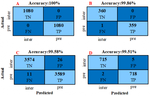
Figure 10. Confusion matrices of the best classification accuracy in channel 8 a) chb07 b) chb17 c) chb01 d) chb02 (pre: preictal, inter: interictal)
The higher AUC values indicated that the system was capable of separating preictal and interictal activities.
The confusion matrices of the best four classifications obtained in channel 8 for segment-based preictal/interictal separation are given in Figure 10. For the classification performed for chb07 using the ResNet model, all the 1080 segments were correctly classified. In the classification performed for chb17, only one out of 360 segments were misclassified. Segment-based classification results for chb01 and chb02 are shown in Figure 10.
Ictal segments are taken into consideration in seizure detection studies, whereas these segments are ignored and a seizure is tried to be determined by comparing preictal and interictal segments in seizure prediction studies. There is no clear procedure to determine preictal activities [2]. The general view is that the preictal interval covers a wide period of time which could be as long as two hours before the onset of a seizure [2, 24, 37]. Accordingly, in the current study, the 30-min interval ending before the onset of seizure was selected as the preictal period. It is important to predict a seizure early enough to allow a clinical intervention [16], which could make the disease more controllable [2].
To date, there have been numerous studies investigating the discrimination of preictal and interictal state. Song et al. proposed a method using the Freiburg data set extracted from 6-channel iEEG recordings of 21 patients. The authors divided the EEG data into parts using 5-second non-overlapping sliding windows from 30-min preictal segments. Using the Sample Entropy properties of each segment, the data was classified as preictal and interictal with 86.75% sensitivity and 83.50% specificity [38].
Lin et al. presented a global feature extraction method from artifact-free EEG segments of 8-channel sEEG data of five patients. Preictal state was selected as the 3-minute section before a seizure onset and the interictal state was selected as the section one hour away from the seizure. The authors used 20-sec overlapping and 30-sec sliding windows and extracted 216 features from each segment. Subsequently, five properties were selected for each patient and the preictal and interictal states were classified with 97.50% accuracy, 96.92% sensitivity, and 97.78% specificity [37].
Cho et al. applied their method for 5-min sEEG recordings of 21 cases in the CHB-MIT dataset. The preictal state was determined as the section 5 minutes before the onset of a seizure and the interictal state was determined as the section 30 minutes away from the seizure. Features were extracted from EEG signals using one-second sliding windows with a band-pass filter, empirical mode decomposition, and filtering algorithms, with an average accuracy of 83.17% [8].
Zhou et al. obtained the iEEG recordings of 21 cases from the Freiburg data set and the sEEG recordings of 23 cases from the CHB-MIT dataset. Both data sets were segmented using a one-second sliding window and were used as input to the 3-layer CNN. EEG data were classified into three different types as preictal/interictal, interictal/ictal and preictal/interictal/ictal. However, the study did not include any information on preictal/interictal selection and a mean accuracy of 95.6%, a mean sensitivity of 94.2%, and mean specificity of 96.6% were achieved in the CHB-MIT dataset [39].
In the method proposed by Elie et al., bispectral properties obtained from 16 channels using iEEG recordings of 3 dogs from the Neurovista data set were used as input to 5-layer ANN. The preictal part consisted of a 5-minute section one hour before the seizure onset, and the interictal state consisted of a 5-minute section four hours away from the seizure. The authors used 30-sec non-overlapping segments for feature extraction and reported that the best testing accuracy obtained for preictal and interictal classification was 78.11% [40].
Tsiouris et al. performed the preictal and interictal differentiation using local and global characteristics from sEEG recording of 24 cases in the CHB-MIT dataset. The preictal state was determined as the section two hours before the seizure onset and the remaining part were determined as the interictal state. The model achieved a sensitivity of 85.75% and a specificity of 85.75% in the classification of preictal and interictal states [2].
Table 6 shows a comparison between the proposed method and those proposed in previously published studies. As shown in Table 6, previous studies determined the preictal interval as the section immediately before the onset of the seizure. In the method proposed in the present study, however, the 30-min interval ending 30 min before the onset of the seizure was selected as the preictal state. Our goal in identifying preictal activities was to examine the predictability of a seizure that could occur at least 30 minutes before the seizure. Another reason was that predicting a seizure 30 minutes earlier is highly important for prompt control of the disease. Our results showed that the preictal region can extend up to one hour before seizure onset. Furthermore, the classification of preictal and interictal states with an accuracy of over 90% showed that the duration of the preictal period showed a wide variation, as reported in previous studies.
Table 6. Comparison between the proposed method and the methods proposed in previous studies
|
Authors |
Methods |
Data |
Preictal interval |
Segments |
Sen |
Spe |
Acc |
|
Song et al. [38] |
Extreme Learning Machine |
21 patients, (Freiburg) |
30min ** |
5 sec, non-overlapping |
86.75 |
83.80 |
- |
|
Lin et al. [37] |
Global features, SVM |
5 patients, (Own dataset) |
3min ** |
30 sec, 20 sec overlapping |
96.92 |
97.78 |
97.50 |
|
Cho et al. [8] |
BPF, EMD, PLV, SVM |
21 patients, (CHB-MIT) |
5min ** |
1 sec, 0.1 sec overlapping |
82.44 |
82.76 |
83.17 |
|
Zhou et al. [39] |
CNN |
23 patients, (CHB-MIT) |
- |
1 sec, non-overlapping |
94.2 |
96.6 |
95.6 |
|
Bou Assi et al. [40] |
Bispectral features, ANN |
3 dogs, (Neurovista) |
5min** |
30 sec, non-overlapping |
- |
- |
78.11 |
|
Tsiouris et al. [2] |
Local & global features, SVM |
24 patients, (CHB-MIT) |
120min ** |
5 sec, non-overlapping |
85.75 |
85.75 |
- |
|
The proposed method |
CNN+SVM |
20 patients, (CHB-MIT) |
30min *** |
5 sec, non-overlapping |
For Channel 8 |
||
|
92.32 |
89.76 |
91.05 |
|||||
** Time before a seizure onset
*** Time set to end 30 minutes before a seizure onset
The advantage of using pre-trained CNN models was that it produced effective features since they were trained on large data set. In this way, more successful classification results can be achieved by using a limited number of training and test data. In doing so, the difficulties in adjusting the hyperparameters in a CNN model design using one-dimensional EEG signals were eliminated. In traditional feature extraction approaches, the extracted features have a significant effect on the classification performance of the system. In these systems, not only the feature extraction process but also the experience of the operator affects the classification performance. Meaningfully, the proposed CNN model was remarkably successful since it extracted features from the data set itself.
The limitation of the study was the prolonged duration of the preictal/interictal interval examined.
In this study, we proposed a method for preictal/interictal recognition, which is an important step for early detection of epileptic seizures, by using EEG signals. In the proposed method, feature extraction was performed from the spectrogram images of EEG signals with pre-trained CNN models, and these features were classified with SVM. Unlike previous studies, the preictal state were determined as the 30-minute interval that ended 30 minutes before the onset of an epileptic seizure. Previous studies have reported that the preictal interval may extend up to two hours before the onset of seizures, and this notion was confirmed by our findings. In the present study, four EEG channels (7, 8, 11, 12) of 20 cases were examined separately. The best classification accuracy for all four channels was obtained in channel 8 (91.05% ± 1.46%) (P3-O1). The mean accuracy of the other three channels was around 90%. These findings suggest that there are significant changes in seizure prediction in the first half an hour period starting 1-h before a seizure occurs. Further studies are needed to contribute to seizure prediction applications and to improve the quality of life of epilepsy patients.
[1] Hussain, L. (2018). Detecting epileptic seizure with different feature extracting strategies using robust machine learning classification techniques by applying advance parameter optimization approach. Cognitive Neurodynamics, 12(3): 271-294. https://doi.org/10.1007/s11571-018-9477-1
[2] Tsiouris, K.M., Pezoulas, V.C., Koutsouris, D.D., Zervakis, M., Fotiadis, D.I. (2017). Discrimination of preictal and interictal brain states from long-term EEG data. 2017 IEEE 30th International Symposium on Computer-Based Medical Systems (CBMS), Thessaloniki, pp. 318-323. https://doi.org/10.1109/CBMS.2017.33
[3] Zhou, W., Liu, Y., Yuan, Q., Li, X. (2013). Epileptic seizure detection using lacunarity and Bayesian linear discriminant analysis in intracranial EEG. IEEE Transactions on Biomedical Engineering, 60(12): 3375-3381. https://doi.org/10.1109/TBME.2013.2254486
[4] Rana, P., Lipor, J., Lee, H., Van Drongelen, W., Kohrman, M.H., Van Veen, B. (2012). Seizure detection using the phase-slope index and multichannel ECoG. IEEE Transactions on Biomedical Engineering, 59(4): 1125-1134. https://doi.org/10.1109/TBME.2012.2184796
[5] Liu, Y., Zhou, W., Yuan, Q., Chen, S. (2012). Automatic seizure detection using wavelet transform and SVM in long-term intracranial EEG. IEEE Transactions on Neural Systems and Rehabilitation Engineering, 20(6): 749-755. https://doi.org/10.1109/TNSRE.2012.2206054
[6] Tafreshi, A.K., Nasrabadi, A.M., Omidvarnia, A.H. (2008). Epileptic seizure detection using empirical mode decomposition. 2008 IEEE International Symposium on Signal Processing and Information Technology, Sarajevo, Bosnia and Herzegovina, pp. 238-242. https://doi.org/10.1109/ISSPIT.2008.4775717
[7] Zhang, Z., Parhi, K.K. (2015). Low-complexity seizure prediction from iEEG/sEEG using spectral power and ratios of spectral power. IEEE Transactions on Biomedical Circuits and Systems, 10(3): 693-706. https://doi.org/10.1109/TBCAS.2015.2477264
[8] Cho, D., Min, B., Kim, J., Lee, B. (2016). EEG-based prediction of epileptic seizures using phase synchronization elicited from noise-assisted multivariate empirical mode decomposition. IEEE Transactions on Neural Systems and Rehabilitation Engineering, 25(8): 1309-1318. https://doi.org/10.1109/TNSRE.2016.2618937
[9] Subasi, A., Gursoy, M.I. (2010). EEG signal classification using PCA, ICA, LDA and support vector machines. Expert Systems with Applications, 37(12): 8659-8666. https://doi.org/10.1016/j.eswa.2010.06.065
[10] Sudalaimani, C., Sivakumaran, N., Elizabeth, T.T., Rominus, V.S. (2019). Automated detection of the preseizure state in EEG signal using neural networks. Biocybernetics and Biomedical Engineering, 39(1): 160-175. https://doi.org/10.1016/j.bbe.2018.11.007
[11] Ibrahim, S., Djemal, R., Alsuwailem, A. (2018). Electroencephalography (EEG) signal processing for epilepsy and autism spectrum disorder diagnosis. Biocybernetics and Biomedical Engineering, 38(1): 16-26. https://doi.org/10.1016/j.bbe.2017.08.006
[12] Tuncer, S.A., Akılotu, B., Toraman, S. (2019). A deep learning-based decision support system for diagnosis of OSAS using PTT signals. Medical Hypotheses, 127: 15-22. https://doi.org/10.1016/j.mehy.2019.03.026
[13] Yildirim, O., Baloglu, U.B., Tan, R.S., Ciaccio, E.J., Acharya, U.R. (2019). A new approach for arrhythmia classification using deep coded features and LSTM networks. Computer Methods and Programs in Biomedicine, 176: 121-133. https://doi.org/10.1016/j.cmpb.2019.05.004
[14] Tan, J.H., Hagiwara, Y., Pang, W., Lim, I., Oh, S.L., Adam, M., Acharya, U.R. (2018). Application of stacked convolutional and long short-term memory network for accurate identification of CAD ECG signals. Computers in Biology and Medicine, 94: 19-26. https://doi.org/10.1016/j.compbiomed.2017.12.023
[15] Lotte, F., Congedo, M., Lécuyer, A., Lamarche, F., Arnaldi, B. (2007). A review of classification algorithms for EEG-based brain–computer interfaces. Journal of Neural Engineering, 4(2): R1. https://doi.org/10.1088/1741-2560/4/2/R01
[16] Acharya, U.R., Hagiwara, Y., Adeli, H. (2018). Automated seizure prediction. Epilepsy & Behavior, 88: 251-261. https://doi.org/10.1016/j.yebeh.2018.09.030
[17] Yıldırım, Ö., Baloglu, U.B., Acharya, U.R. (2018). A deep convolutional neural network model for automated identification of abnormal EEG signals. Neural Computing and Applications, 32: 15857-15868. https://doi.org/10.1007/s00521-018-3889-z
[18] Toraman, S., Tuncer, S.A., Balgetir, F. (2019). Is it possible to detect cerebral dominance via EEG signals by using deep learning? Medical Hypotheses, 131: 109315. https://doi.org/10.1016/j.mehy.2019.109315
[19] Ullah, I., Hussain, M., Aboalsamh, H. (2018). An automated system for epilepsy detection using EEG brain signals based on deep learning approach. Expert Systems with Applications, 107: 61-71. https://doi.org/10.1016/j.eswa.2018.04.021
[20] Fahimi, F., Zhang, Z., Goh, W.B., Lee, T.S., Ang, K.K., Guan, C. (2019). Inter-subject transfer learning with an end-to-end deep convolutional neural network for EEG-based BCI. Journal of Neural Engineering, 16(2): 026007. https://doi.org/10.1088/1741-2552/aaf3f6
[21] Supratak, A., Dong, H., Wu, C., Guo, Y. (2017). DeepSleepNet: A model for automatic sleep stage scoring based on raw single-channel EEG. IEEE Transactions on Neural Systems and Rehabilitation Engineering, 25(11): 1998-2008. https://doi.org/10.1109/TNSRE.2017.2721116
[22] Oh, S.L., Hagiwara, Y., Raghavendra, U., Yuvaraj, R., Arunkumar, N., Murugappan, M., Acharya, U.R. (2018). A deep learning approach for Parkinson’s disease diagnosis from EEG signals. Neural Computing and Applications, 32: 10927-10933. https://doi.org/10.1007/s00521-018-3689-5
[23] CHB-mit scalp EEG database, Physionet.org. Available: https://www.physionet.org/pn6/chbmit, accessed on 12 August 2020.
[24] Alotaiby, T.N., Alshebeili, S.A., Alotaibi, F.M., Alrshoud, S.R. (2017). Epileptic seizure prediction using CSP and LDA for scalp EEG signals. Computational Intelligence and Neuroscience, 2017: 1-11. https://doi.org/10.1155/2017/1240323
[25] Truong, N.D., Nguyen, A.D., Kuhlmann, L., Bonyadi, M.R., Yang, J., Kavehei, O. (2017). A generalised seizure prediction with convolutional neural networks for intracranial and scalp electroencephalogram data analysis. arXiv preprint arXiv:1707.01976.
[26] Baloglu, U.B., Talo, M., Yildirim, O., San Tan, R., Acharya, U.R. (2019). Classification of myocardial infarction with multi-lead ECG signals and deep CNN. Pattern Recognition Letters, 122: 23-30. https://doi.org/10.1016/j.patrec.2019.02.016
[27] Krizhevsky, A., Sutskever, I., Hinton, G.E. (2012). ImageNet classification with deep convolutional neural networks. Proceedings of the 25th International Conference on Neural Information Processing Systems, pp. 1097-1105. https://doi.org/10.1145/3065386
[28] Yildirim, O., Talo, M., Ay, B., Baloglu, U.B., Aydin, G., Acharya, U.R. (2019). Automated detection of diabetic subject using pre-trained 2D-CNN models with frequency spectrum images extracted from heart rate signals. Computers in Biology and Medicine, 113: 103387. https://doi.org/10.1016/j.compbiomed.2019.103387
[29] Gopalakrishnan, K., Khaitan, S.K., Choudhary, A., Agrawal, A. (2017). Deep convolutional neural networks with transfer learning for computer vision-based data-driven pavement distress detection. Construction and Building Materials, 157: 322-330. https://doi.org/10.1016/j.conbuildmat.2017.09.110
[30] Simonyan, K., Zisserman, A. (2014). Very deep convolutional networks for large-scale image recognition. arXiv preprint arXiv:1409.1556.
[31] Zagoruyko, S., Komodakis, N. (2016). Wide residual networks. arXiv preprint arXiv:1605.07146.
[32] He, K., Zhang, X., Ren, S., Sun, J. (2016). Deep residual learning for image recognition. 2016 IEEE Conference on Computer Vision and Pattern Recognition (CVPR), Las Vegas, NV, pp. 770-778. https://doi.org/10.1109/CVPR.2016.90
[33] Huang, G., Liu, Z., Van Der Maaten, L., Weinberger, K.Q. (2017). Densely connected convolutional networks. 2017 IEEE Conference on Computer Vision and Pattern Recognition (CVPR), Honolulu, HI, pp. 2261-2269. https://doi.org/10.1109/CVPR.2017.243
[34] Toraman, S., Girgin, M., Üstündağ, B., Türkoğlu, İ. (2019). Classification of the likelihood of colon cancer with machine learning techniques using FTIR signals obtained from plasma. Turkish Journal of Electrical Engineering & Computer Sciences, 27(3): 1765-1779. https://doi.org/10.3906/elk-1801-259
[35] Khazaee, A., Ebrahimzadeh, A. (2010). Classification of electrocardiogram signals with support vector machines and genetic algorithms using power spectral features. Biomedical Signal Processing and Control, 5(4): 252-263. https://doi.org/10.1016/j.bspc.2010.07.006
[36] Yang, Y., Zhou, M., Niu, Y., Li, C., Cao, R., Wang, B., Xiang, J. (2018). Epileptic seizure prediction based on permutation entropy. Frontiers in Computational Neuroscience, 12: 55. https://doi.org/10.3389/fncom.2018.00055
[37] Lin, L.C., Chen, S.C.J., Chiang, C.T., Wu, H.C., Yang, R.C., Ouyang, C.S. (2017). Classification preictal and interictal stages via integrating interchannel and time-domain analysis of EEG features. Clinical EEG and Neuroscience, 48(2): 139-145. https://doi.org/10.1177/1550059416649076
[38] Song, Y., Zhang, J. (2016). Discriminating preictal and interictal brain states in intracranial EEG by sample entropy and extreme learning machine. Journal of Neuroscience Methods, 257: 45-54. https://doi.org/10.1016/j.jneumeth.2015.08.026
[39] Zhou, M., Tian, C., Cao, R., Wang, B., Niu, Y., Hu, T., Xiang, J. (2018). Epileptic seizure detection based on EEG signals and CNN. Frontiers in Neuroinformatics, 12: 95. https://doi.org/10.3389/fninf.2018.00095
[40] Bou Assi, E., Gagliano, L., Rihana, S., Nguyen, D.K., Sawan, M. (2018). Bispectrum features and multilayer perceptron classifier to enhance seizure prediction. Scientific Reports, 8(1): 1-8. https://doi.org/10.1038/s41598-018-33969-9