Zhe Li* | Xiao Han | Liya Wang | Tongyi Zhu | Futian Yuan
© 2020 IIETA. This article is published by IIETA and is licensed under the CC BY 4.0 license (http://creativecommons.org/licenses/by/4.0/).
OPEN ACCESS
Facing the existing digital image libraries on landscape, researchers need to urgently solve a challenging problem: how to realize rational management and accurate retrieval of landscape images that contain feature information like hierarchy, layout, color system, and color matching. For accurate organization and labeling of landscape Images, this paper presents a novel method for feature extraction and image retrieval of landscape images based on image processing. Firstly, a color quantization process was designed for landscape images, and used to analyze the color composition and color space pattern (CSP) of such images. Next, the existing methods, which are suitable for the extraction of color features from landscape Images, were briefly reviewed, and the basic flows of our improved algorithm and division method of landscape color blocks (LCBs) were explained. Finally, the retrieval performance of landscape images was improved by matching of weighted color blocks of regional landscape, based on the multi-dimensional color eigenvectors of landscape image. The experimental results demonstrate the effectiveness of our algorithm. The research results shed light on the feature extraction from other types of color images.
landscape image, color feature extraction, image retrieval, image processing
Landscape images provide the most intuitive and accurate expression of landscape, by feat of the various carriers of characteristic information, such as hierarchy, layout, color system, and color matching [1-3]. Facing the existing digital image libraries with the theme of landscape design, researchers need to urgently realize the management and retrieval of landscape images, based on their understanding of image attributes (texture and color) and image contents (hierarchy) [4-7]. By the current classification criteria, the landscape image databases mainly include images in the following categories: garden architecture, garden landscaping, garden plant landscape, and garden artworks [8-10]. The effective retrieval and use of landscape images depend on accurate image organization and labeling, which require the extraction of features by class features and image pattern.
Landscape design covers the construction of such elements as terrain, water body, and architecture [11]. Many scholars at home and abroad have explored landscape planning and design based on image processing [12-14]. Zhang [15] stressed that plant landscape is now the most important means to express landscape, due to the growing awareness of ecology and environment, collected a massive amount of landscape images through field surveys, and expounded the basic features of the physical elements in landscape space in the aspects of spatial form, subject type, hierarchical structure, color matching, and subject combination. Through comparative and case analyses, Wangda et al. [16] examined the structure of landscape in a top-down manner based on satellite images, and summarized the planning focuses for landscapes with different design styles: landscape gardens, modern gardens, and renaissance gardens. Li et al. [17] treated color as an important carrier of the artistry of landscapes, and proposed to realize the expressiveness and identifiability of landscape images through good color planning and design.
Some scholars have investigated image processing methods involving ancient buildings or classical landscapes. Lang et al. [18] designed an analysis method for ancient town landscapes with aging buildings and fuzzy features; By quantifying the grayscale features of remote sensing images, the designed method achieves a high accuracy in extracting image features. Based on genetic algorithm and quadrature mirror filter, Smutnicki [19] put forward a visual effect optimization method to overcome the low resolution and severe information loss of classical landscape images, and proved that the method can output high resolution images and extract desirable image features. Elfadaly et al. [20] combined the histogram equalization with the imaging mechanism into a hybrid strategy: Firstly, the salient areas in each fuzzy landscape image are equalized; the contrast difference vectors of the salient areas are acquired by histogram specification; the difference vectors were optimized to reconstruct an enhanced image.
On account of the rich color changes, the space of the landscape has a sense of hierarchy and dynamic beauty. The research into the color combination, color contrast, and color attribute quantization of landscape images greatly benefits the feature extraction from such images [21-24]. From the perspectives of leaf color, flower color, fruit color, and branch color, Zhang and Li [25] explored the principles and methods of color matching for landscape plants, and summed up the color features of plant communities for landscape images in different seasons. Mulvihill et al. [26] discussed the rational use of landscape plant colors from the angle of design techniques, and suggested that the artistic beauty of landscapes should focus on the diversity, unity, and balance of colors and patterns.
The feature extraction of landscape images is the key to the image retrieval and classification based on attributes and contents. The feature extraction of landscape images can be completed by describing the high-level image semantics with the unique feature information like spatial color matching and hierarchy. Therefore, this paper presents a novel method for feature extraction and image retrieval of landscape images based on image processing.
The remainder of this paper is organized as follows: Section 2 presents the color quantization flow and introduces the analysis method for color composition and color space pattern (CSP); Section 3 briefly reviews the existing methods suitable for the extraction of color features from landscape images, explains the basic flow of our improved algorithm, and details the division of landscape color blocks (LCBs); Section 4 improves the retrieval performance of landscape images through the matching of weighted color blocks of regional landscape, based on the multi-dimensional color eigenvectors of landscape images; Section 5 proves the effectiveness of our algorithm through experiments; Section 6 summarizes the main findings of this research.
Figure 1. The color quantization of landscape images
The extraction of color features is the key to the retrieval of landscape images. Before feature extraction, it is necessary to quantify the complex color composition. Figure 1 details the process of color quantization. Firstly, the interferences were removed from the original image on Photoshop, and the RGB color space was transformed to the HSV color space on MATLAB. The RGB-HSV transform can be expressed as:
$\left\{ \begin{align} & {R}'=\frac{R}{255},{G}'=\frac{G}{255},{B}'=\frac{B}{255} \\ & V=\frac{{R}'+{G}'+{B}'}{3} \\ & H={{90}^{\circ }}-\arctan \left( \frac{2R'-G'-B'}{\sqrt{3}\left( G'-B' \right)} \right)\times \frac{{{180}^{\circ }}}{\pi } \\ & +\left\{ 0,G'>B';G'<B' \right\} \\ & s=1-\frac{\min \left( R',G',B' \right)}{V} \\ \end{align} \right.$ (1)
Then, the components of hue H, saturation S, and value V were uniformly quantized at non-equal intervals. The value of H falls into the range of [0, 360]. The H value can be quantized by:
${{H}_{UQ}}=\left\{ \begin{align} & 0,\text{ }310\le H\le 360\text{ or }0\le H<25 \\ & 1,\text{ }25\le H<50 \\ & 2,\text{ }50\le H<75 \\ & 3,\text{ }75\le H<160 \\ & 4,\text{ }160\le H<200 \\ & 5,\text{ }200\le H<280 \\ & 6,\text{ }280\le H<295 \\ & 7,\text{ }295\le H<310 \\ & 8,\text{ }S=0\text{ }and\text{ }V=3 \\ & 9,\text{ }S=0\text{ }and\text{ }V=1\text{ }or\text{ }V=2 \\ & 10,\text{ }V=0 \\ \end{align} \right.$ (2)
If S and V take extreme values (0 or 1), some pixels in the landscape image will become white, gray, or black. The hue is red, orange, yellow, green, cyan, blue, purple, amaranth, white, gray, and black, respectively, when HUQ is 0, 1, 2, 3, 4, 5, 6, 7, 8, 9, and 10. The value of S falls into the range of [0, 1]. The S value can be quantized by:
${{S}_{UQ}}=\left\{ \begin{align} & 0,0\le S<0.16 \\ & 1,0.16\le S<0.45 \\ & 2,0.45\le S<0.80 \\ & 3,0.80\le S<1 \\ \end{align} \right. $ (3)
The saturation is ultralow, low, moderate, and high, respectively, when SUQ is 0, 1, 2, and 3. The value of V falls into the range of [0, 1]. The V value can be quantized by:
$ {{V}_{UQ}}=\left\{ \begin{align} & 0,0\le V<0.16 \\ & 1,0.16\le V<0.45 \\ & 2,0.45\le V<0.8 \\ & 3,0.8\le V<1 \\ \end{align} \right.$ (4)
The value is ultralow, low, moderate, and high, respectively, when VUQ is 0, 1, 2, and 3. Then, the extreme values of S and V were normalized for white, gray, and black. After normalization, the 180 uniformly quantized colors could be reduced to 88.
The color features of landscape images were characterized by color composition and CSP. Let HUQ-i, SUQ-i, and VUQ-i be the number of image pixels occupied by the i-th hue, saturation, and value, respectively. These parameters can reflect the color composition of the original image. Then, the proportions of HUQ-i, SUQ-i, and VUQ-i in the total number P of pixels can be respectively expressed by:
$\left\{\begin{array}{l}D_{H-i}=\frac{H_{U Q-i}}{P} \\ D_{S-i}=\frac{S_{U Q-i}}{P} \\ D_{V-i}=\frac{V_{U Q-i}}{P}\end{array}\right.$ (5)
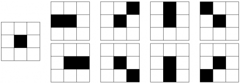
The CSP was characterized by the attributes of LCBs divided by hue. Figure 2 provides an example of the analysis of the CSP of landscape. Obviously different LCBs correspond to different landscape levels. To analyze the CSP, eight indices were selected for separate analysis: the number of color blocks, the area of the largest color block, the shape index of color blocks, the spread of color, the separation of color, the diversity of color, the uniformity of color, and the aggregation of color.
Figure 2. An example of the analysis of the CSP of landscape
3.1 Extraction methods
Currently, there are three suitable extraction methods for color features from landscape images.
(1) Color moment
The color moment capable of characterizing the CSP and pixel correlations can be computed by:
$\left\{ \begin{matrix} {{M}_{\text{mea-}i}}=\frac{1}{P}\sum\limits_{j=1}^{P}{{{H}_{ij}}} \\ {{M}_{\operatorname{var}\text{-}i}}=\sqrt{\left( \frac{1}{P}\sum\limits_{j=1}^{P}{{{\left( {{H}_{ij}}-{{M}_{\text{mea-}i}} \right)}^{2}}} \right)} \\ {{M}_{\text{ske-}i}}=\sqrt{\left( \frac{1}{P}\sum\limits_{j=1}^{P}{{{\left( {{P}_{ij}}-{{M}_{\text{mea-}i}} \right)}^{3}}} \right)} \\\end{matrix} \right.$ (6)
where, Hij is the i-th hue component of the j-th pixel. Without sufficient depiction of the CSP, this method needs to be combined with other feature extraction methods, in order to reduce the range of image retrieval.
(2) Color aggregation vector
The color aggregation vector overcomes the defect of the color moment. The vector can be calculated by:
$A=\left\{ \left( {{x}_{1}},{{y}_{1}} \right),\left( {{x}_{\text{2}}},{{y}_{\text{2}}} \right),\ldots ,\left( {{x}_{P}},{{y}_{P}} \right) \right\}$ (7)
where, xi and yi are the number of aggregated color pixels and that of non-aggregated color pixels in the i-th LCB in the color image histogram, respectively. To prevent all LCBs with the same hue from being judged as aggregated or non-aggregated, formula (7) can be improved as:
${A}'=\left\{ \left( {{c}_{1}},{{{{x}'}}_{1}},{{{{y}'}}_{1}} \right),\left( {{c}_{2}},{{{{x}'}}_{2}},{{{{y}'}}_{2}} \right),\ldots ,\left( {{c}_{n}},{{{{x}'}}_{n}},{{{{y}'}}_{n}} \right) \right\}$ (8)
where, ci is the center value of the i-th LCB; x'i and β'i are the number of pixels in the i-th LCB judged as aggregated and non-aggregated, respectively. If ci is greater than the preset threshold, the corresponding pixel is aggregated; if ci is smaller than that threshold, the corresponding pixel is not aggregated.
(3) Local correlation-based method
Before retrieval, the color features of the original landscape image must be rotatable, translatable, and scale-invariant. The image feature extraction algorithm, which is based on local correlations of color retrieval, integrates the retrieval representation of the color histogram with the quantized values of image colors, and obtains rich color textures with a light computing load.
This local correlation-based method first transforms the three dimensions of HSV color space, i.e. H, S, and V, into an R-dimensional retrieval matrix {X1,X2,…,XR}, and then computes the 0th- and 1st-order correlations between matrix elements by:
$\left\{ \begin{matrix} {{\text{0}}^{th}}\text{: }{{q}_{0}}\left( k \right)=\sum\limits_{\tau \in \Omega }{{{X}_{k}}\left( \tau \right)} \\ {{\text{1}}^{st}}:\text{ }{{q}_{kl}}\left( k,l,\varepsilon \right)=\sum\limits_{\tau \in \Omega }{{{X}_{k}}\left( \tau \right)}{{X}_{l}}\left( \tau +\varepsilon \right) \\\end{matrix} \right.$ (9)
Figure 3. The workflow of the improved algorithm for image feature extraction
However, the local correlation-based method tends to overlook the detailed features of local colors. To solve the defect, this paper prepares an improved algorithm for image feature extraction, whose workflow is explained in Figure 3.
First, N pixels were selected from the landscape image color space to represent the basic color attributes. The weights of these pixels were taken as the basis for image color retrieval. Figure 4 shows the pixles selected from cubic and conic color spaces.
(a)
(b)
Figure 4. The pixels selected from cubic (a) and conic (b) color spaces
The weight of the color attribute Cp=(H,S,V) for any pixel on the image can be computed by:
$\begin{align} & {{p}_{C}}=V\left( 1-S \right)White+\left( 1-V \right)Black \\ & +VS\frac{{{H}_{2}}-H}{{{H}_{2}}-{{H}_{1}}}{{C}_{1}}+VS\frac{H-{{H}_{1}}}{{{H}_{2}}-{{H}_{1}}}{{C}_{2}} \\ \end{align}$ (10)
where, White is white color; Black is block color; C1 and C2 are two color attributes on the top circle of the conic color space, which are the most similar to Cp; H1 and H2 are the hue values at the pixels corresponding to C1 and C2, respectively; H is a hue value between H1 and H2.
The weights (Black, White, C1, C2) of the most similar R basic color attributes were combined into a sparse matrix {X1,X2,…,XR}, which represents the target landscape image. The matrix element Xk is the color descriptor of the image.
The CSP of the landscape image was mainly measured by the correlation between the basic color attribute distributions of any two pixels. Let ε be the displacement vector of a pixel pointing to the reference point, that is, the color space interval between two pixels. Then, ε could be defined as ε={Δτ,0), (Δτ,Δτ), (0,Δτ), (-Δτ,Δτ)} based on the symmetry of spatial positions. To acquire more detailed features of image colors, the unit pixel interval Δτ was set to 1. The 0th and 1st-order correlations of Xk can be respectively calculated by:
$\left\{ \begin{matrix} {{\text{0}}^{th}}\text{: }{{q}_{0}}\left( k \right)=\sum\limits_{\tau \in \Omega }{{{X}_{k}}\left( \tau \right)} \\ \begin{align} & \text{ }{{\text{1}}^{st}}:\text{ }{{q}_{kl}}\left( k\le l \right)=\sum\limits_{\tau \in \Omega }{{{X}_{k}}\left( \tau \right)}{{X}_{l}}\left( \tau \right) \\ & \text{ }q\left( k,\varepsilon ,\tau \right)={{X}_{k}}\left( \tau \right){{X}_{k}}\left( \tau +\varepsilon \right) \left( \tau \in {{\Omega }_{i}}\text{ }i\in \left[ \text{1,}I \right] \right) \\ \end{align} \\\end{matrix} \right.$ (11)
where, Ωi is the i-th LCB of the landscape image; I is the total number of LCBs. The above analysis shows that, the 0th-order correlation computation of the traditional color histogram produces a 1×R-dimensional color feature FEA0, which represents the distribution law of the R basic color attributes of the entire landscape image; the 1st-order correlation computation of the i-th LCB of the landscape image produces a 1×[(R-1)+(R-2)+…+1]-dimensional color feature FEA1i, which represents the color features of the i-th LCB.
The local details of LCB color distribution could be obtained by calculating the color correlation between two pixels, using FEA1i; meanwhile, the variation in CLI color space could be derived from ε by computing the color space interval. The two calculations are both based on pixel information. To mitigate the redundancy of local information, the distribution law of R basic color attributes was statistically optimized in s different directions within Ωi:
$ q\left( k,\varepsilon \right)=\sum\limits_{\tau \in {{\Omega }_{i}}}{q\left( k,\varepsilon ,\tau \right)}$ (12)
The distribution law of formula (12) was recorded as CLI color feature FEA2i. Figure 5 compares the statistical directions of the distribution laws for basic color attributes before and after optimization.
(a) (b)
Figure 5. The statistical directions of the distribution laws for basic color attributes before (a) and after (b) optimization
The local color features thus obtained are more detailed than those extracted by the local correlation-based method. To sum up, the R+[(R-1)+(R-2)+…+1]+R×s}×I-dimensional color feature of the landscape image obtained by the improved algorithm can be expressed as:
$FEA=\left\{ \begin{align} & FE{{A}_{0}};FE{{A}_{01}},\ldots ,FE{{A}_{0I}}; \\ & FE{{A}_{21}},\ldots ,FE{{A}_{2I}} \\ \end{align} \right\}$ (13)
Despite containing details on the local color distribution of landscape image LCBs, FEA1i and FEA2i emphasize the basic color attributes over color distribution law. To solve the problem, formula (11) can be optimized as:
$\begin{align} & q\left( \varepsilon ,\tau \right)=\sum\limits_{\tau \in \Omega }^{R}{{{X}_{k}}\left( \tau \right){{X}_{k}}\left( \tau +\varepsilon \right)} \\ & \left( \tau \in {{\Omega }_{i}}\text{ }i\in \left[ \text{1,}I \right] \right) \\ \end{align}$ (14)
Formula (14) shows the correlation between the (τ, τ+ε) color distribution laws of two pixels under s different neighboring directions. q(ε,τ) is a constant within [0, 1]. The smaller the s value, the weaker the color distribution laws between the two pixels, and the larger the color gap between them. Here, the value range of q(ε,τ) is divided into 9 intervals T1~T9, where T1=[0,0.15], T9=(0.85,l], and T2~T8 are equally divided intervals of (0.15,0.85]. Then, the number of q(ε,τ) values that belong to each interval was counted. The resulting 9×s-dimensional image color feature was recorded as FEA'2i:
$FE{{{A}'}_{2i}}\left( u,\varepsilon \right)=Sta\left( q\left( \varepsilon ,\tau \right)\in {{T}_{u}} \right)$ (15)
The invariance of the value interval of q(ε,τ) guarantees that the color features of the final image do not change with the image size or color. Then, formula (13) can be optimized as:
$FE{A}'=\left\{ \begin{align} & FE{{A}_{0}};FE{{A}_{11}},\ldots ,FE{{A}_{1I}}; \\ & FE{{{{A}'}}_{21}},\ldots ,FE{{{{A}'}}_{2I}} \\ \end{align} \right\}$ (16)
Hence, FEA’ has a dimension of R+[(R-1)+(R-2)+…+1]+9×s}×I.
3.2 LCB division
The LCBs of the landscape image were divided in the following process. Let pE be the set of edge pixels in color features of the landscape image. First, the quantization center (xc, yc) of the color features was determined. Next, the color feature pixels of the image were reconstructed. After that, the image was processed by the smoothing filter to approximate the color difference feature:
$\overline{FE{{A}_{i}}}=\frac{1}{E}\sum\limits_{i=1}^{I}{{{B}_{i}}}$ (17)
where, B1,B2,B3…Bi are the sub-features of each LCB; E is the feature component of landscape image color edges. Then, a spatial distribution model was constructed for multiple pixels with basic color features, and the statistical shape model for the entire landscape image was built by grayscale quantization. In this way, the two neighboring pixel sets can be obtained as:
$\begin{align} & PS=\tilde{h}\left( x,y \right)=h\left( x,y \right)\sqrt{\frac{r\left( x \right)}{r\left( y \right)}} \\ & =\frac{g\left( x,y \right)}{r\left( x \right)}\sqrt{\frac{r\left( x \right)}{r\left( y \right)}}=\frac{g\left( x,y \right)}{\sum\limits_{y}{g\left( x,y \right)}}\sqrt{\frac{\sum\limits_{y}{g\left( x,y \right)}}{\sum\limits_{x}{g\left( x,y \right)}}} \\ \end{align}$ (18)
where, g(x, y) is the gray pheromone value of the pixel. The g(x, y) was extracted from the landscape image color eigenvector through sparse linear segmentation, producing the matching template of the first v-dimensional color features. Let θLTM be the matching template of local color features, and EHSV be the feature component of color edges of the landscape image. Based on the extracted color features, the LCBs of the landscape image were recognized automatically. Then, the edge feature points of each LCB were enhanced and pinpointed rapidly through neighborhood search:
$E\left( g(x,y) \right)=\frac{1}{2}\left( \begin{align} & {{\left| Z-\left| \sum\limits_{y}{g\left( x,y \right)}-\sum\limits_{X}{g\left( x,y \right)} \right| \right|}^{2}} \\ & +\lambda \sqrt{\left| \begin{align} & {{\sum\limits_{y}{g\left( x,y \right)}}^{2}}+2\sum\limits_{y}{g\left( x,y \right)} \\ & \sum\limits_{x}{g\left( x,y \right)}+\sum\limits_{x}{g{{\left( x,y \right)}^{2}}} \\ \end{align} \right|} \\ \end{align} \right)$ (19)
The edges of the landscape image were reset, and the sparse linear equation set was constructed for the corresponding color attributes. By edge detection method, the textures of the landscape image colors were segmented to obtain the distribution law of gray pixel features:
$Z=\frac{1}{m}\sum\limits_{i=0}^{m-1}{\left| \sum\limits_{y}{g\left( x,y \right)}-\sum\limits_{X}{g\left( x,y \right)} \right|}$ (20)
where, m is the number of pixels of the target LCB. The LCB edge features that carry the characteristics of human vision were extracted, and the template matching coefficient θLTM was configured. Then, the edge eigenvectors of each LCB were denoted as FEAE and FEA'E. The global color features and LCB division method of the entire landscape image have nothing to do with weight setting. Next, the feature weight ω was introduced to reflect the regional difference of LCBs. The edge features of the corresponding LCB can be expressed as:
$\left\{\begin{array}{l}F E A=\left\{\begin{array}{l}F E A_{0} ; \omega_{11} F E A_{11}, \ldots, \omega_{1 I} F E A_{1 I} \\ \omega_{21} F E A_{21}, \ldots, \omega_{2 I} F E A_{2 I}\end{array}\right\} \\ F E A^{\prime}=\left\{\begin{array}{l}F E A_{0} ; \omega_{11} F E A_{11}, \ldots, \omega_{1 I} F E A_{1 I} \\ \omega_{21}^{\prime} F E A_{21}^{\prime}, \ldots, \omega_{2 I}^{\prime} F E A_{2 I}^{\prime}\end{array}\right\}\end{array}\right.$ (21)
where, ω11+ω12+…+ω1I=1; ω21+ω22+…+ω2I=1; ω'21+ω'22+…+ω'2I=1. The value of feature weight ω shows the significance of the edge features of the LCB to the color features of the entire landscape image.
To further optimize the retrieval effect on the landscape image, the weighted regional LCB matching was performed based on the multi-dimensional color eigenvector of the landscape image. Let F and Fd be the target landscape image and the d-th image to be matched in the library, respectively; M and Md are the number of LCBs in the landscape image and the d-th image, respectively. Once the sub-features of LCBs were extracted, the LCB color feature sequences of F and Fd can be respectively described as:
$\left\{ \begin{matrix} B=\left\{ B_{1}^{{}},B_{2}^{{}},\ldots ,B_{I}^{{}} \right\} \\ {{B}^{d}}=\left\{ B_{1}^{d},B_{2}^{d},\ldots ,B_{I}^{d} \right\} \\\end{matrix} \right.$ (22)
The feature distance from the sub-feature Bi in the i-th LCB of F to the sub-feature Bdi in the j-th LCB of Fd can be calculated by:
$DIS_{ij}^{d}=\left\| B_{i}^{{}}-B_{j}^{d} \right\|,0\le i\le M,0\le j\le {{M}^{d}}$ (23)
All feature distances were allocated to the same set Ddi={DISdi1,DISdi2,…,DISdiMd}. The optimal color of Bi was defined as the minimum value in the set:
$DI{{{S}'}_{i}}=\underset{0\le j\le {{M}^{d}}}{\mathop{\min }}\,DIS_{ij}^{d}$ (24)
The optimal color feature distances have one-to-one correspondence with the LCBs. Then, F and Fd have a set of optimal color feature distances, which are denoted as DISbest={DIS'1, DIS'2, …, DIS'M} and DISdbest={DIS'd1, DIS'd2 ,…, DIS'dM}, respectively. The similarity between F and Fd was defined as the sum of the weighted mean of optimal color feature distances in DISbest and DISdbest:
$\operatorname{SIM}\left(B, B^{d}\right)=\frac{1}{M} \sum_{i=1}^{M} \delta_{i} D I S_{i}^{\prime}+\frac{1}{M^{d}} \sum_{j=1}^{M^{d}} \delta_{j}^{d} D I S_{j}^{\prime d}$ (25)
where, δi and δdi are the proportions of the i-th LCB of F and the j-th LCB of Fd in the total area of the landscape image, respectively. The two parameters measure the importance of different LCBs to image color features.
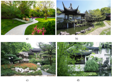
The cases of our experiments are the landscape images that reflects the concept and artistic conception of Chinese landscape painting. As shown in Figure 6, four landscape images with different hierarchies and landscape layouts were subject to color quantization, before being analyzed for color composition and CSP.
Figure 6(a) is a plant-dominated CLI with a high value contrast. The foreground consists of dark green herbs and shrubs, while the background involves light green small and large trees. The CLI is also embellished by red and yellow colors. Figures 6(b)-(d) are all landscapes that intermingle red and green plants with the antique colors of Huizhou and Suzhou gardens. The balanced arrangement of ornamental colors leads to a good color appearance in the three landscape images.
Figure 6. The target CLIs for color quantization
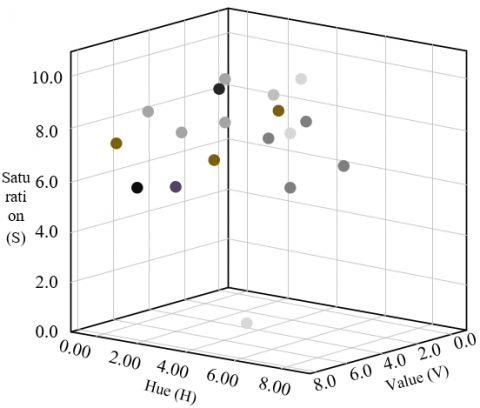
The colors of the three landscape images that intermingle plant landscape with architectural landscape were quantified. The quantified colors are displayed in Figure 7. Figure 7(a) is the scatterplot of plant landscape colors. The color composition of the plant landscape exhibited a moderate to low saturation and a low value; the overall composition was stable, with a good texture. Figures 7(b) and (c) provide the scatter points of colors of walls, and specific structures (e.g., columns, doors, and windows). It can be seen that the hue of walls and saturation of specific structures in architectures were distributed in a concentrated manner; the colors were dark gray; the color composition was of moderate value, and moderate to low hue; the color diversity was not high, possibly due to the architectural style of the landscape.
(a)
(b)
(c)
Figure 7. The scatterplots of landscape image colors
(a)
(b)
Figure 8. The color composition of the landscape images in different periods
Table 1. The correlations with CSP characteristic elements
|
|
Number of color blocks |
Area of the largest color block |
Shape index |
Spread |
Separation |
Diversity |
Uniformity |
Aggregation |
|
Number of color blocks |
1 |
|
|
|
|
|
|
|
|
Area of the largest color block |
-0.7422** |
1 |
|
|
|
|
|
|
|
Shape index |
-0.2238 |
0.3463 |
1 |
|
|
|
|
|
|
Spread |
-0.4726* |
-0.3665* |
0.1641 |
1 |
|
|
|
|
|
Separation |
0.05411 |
0.1742 |
-0.0413 |
0.0842 |
1 |
|
|
|
|
Diversity |
0.5121* |
-0.2983 |
0.2745 |
-0.3425* |
-0.2244 |
1 |
|
|
|
Uniformity |
0.1742 |
0.1765 |
0.0547 |
-0.4875* |
0.5453* |
-0.4215* |
1 |
|
|
Aggregation |
-0.3748 |
-0.1844 |
-0.3597 |
-0.0143 |
-0.2742 |
-0.2245 |
0.1148 |
1 |
Table 2. The correlations of relative height of color space with some characteristic elements
|
|
Spread |
Separation |
Diversity |
Uniformity |
Aggregation |
|
Relative height of color space |
-0.1214 |
0.3419 |
0.1943 |
0.5470 |
0.3424 |
Table 3. The correlations of relative height of color space with foreground/background attributes
|
|
Area of foreground color blocks |
Shape index of foreground color blocks |
Area of background color blocks |
Shape index of background color blocks |
Area ratio of foreground to background color blocks |
|
Relative height of color space |
0.4165 |
0.2441 |
0.4513 |
-0.1324 |
0.2022 |
Table 4. The image retrieval results after two optimizations under different number of LCBs
|
Image area |
Post-first optimization |
Post-second optimization |
||
|
Number of LCBs |
Mean precision |
Color feature dimension |
Mean precision |
Color feature dimension |
|
No division |
51.24% |
56 |
84.13% |
88 |
|
6 color blocks |
68.24% |
138 |
86.33% |
258 |
|
12 color blocks |
74.35% |
276 |
87.47% |
376 |
|
16 color blocks |
81.74% |
356 |
91.62% |
468 |
Figure 8 presents the color composition of the same landscape in different periods. It could be observed that, the color composition of the image on the same landscape followed the following distribution laws in different periods: the saturation and value were moderate; green was the dominant color, supplemented by black, white, and gray; the proportions of red, orange, and yellow slightly changed with the variation in landscape temperature.
The data on eight indices for CSP analysis, including the number of color blocks, the area of the largest color block, the shape index of color blocks, the spread of color, the separation of color, the diversity of color, the uniformity of color, and the aggregation of color, were permutated and combined. Table 1 records the results of correlation analysis on CSP characteristic elements. Table 2 provides the results of correlation analysis on relative height of color space and some characteristic elements. It can be seen that the relative height of color space, which reflects spatial openness, has a significant positive correlation with the separation, uniformity, and aggregation of image colors, a negative correlation with spread, and a weak correlation with diversity.
Table 3 presents the results on the correlation analysis on relative height of color space and foreground/background attributes. It can be learned that the relative height of color space has a significant positive correlation with the color block size in the foreground and background, a negative correlation with shape index of foreground color blocks, and a weak correlation with diversity.
In this paper, the distribution laws of basic color attributes are collected in different directions, and special consideration is given to the correlation between color distributions. After these two optimizations, the mean precisions and color feature dimensions at different number of color blocks were summarized in Table 4. It is clear that our LCB division method effectively increased the retrieval efficiency of the landscape image by extracting the color eigenvectors. However, the division of an excessive number of color blocks increased the feature dimension, making the computation more complex.
After analyzing the color composition and CSPs of the landscape images, the influence of our LCB division method on image retrieval was measured by mean precision through contrastive experiments. Figure 9 displays the image retrieval results by different LCB division methods. With the growing area of the LCB, the precision of image retrieval decreased. The number of LCBs must be determined as that corresponding to the optimal retrieval results. In general, the image retrieval method that considers the distribution law of colors achieved the better precision.
Figure 9. The image retrieval results by different LCB division methods
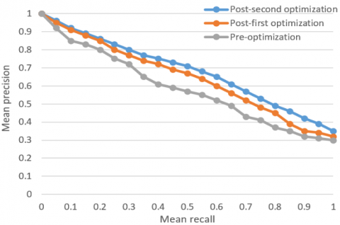
Figure 10. The image retrieval results of our improved algorithm
The image retrieval results of our improved algorithm in shown in Figure 10. It can be seen that our algorithm achieved a good retrieval results on landscape images. The retrieval curve after the second optimization was better than that before optimization.
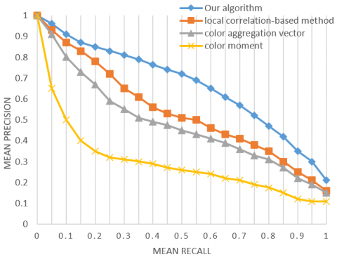
Finally, different image feature extraction algorithms were separately applied to retrieve the several landscape image sets. As shown in Figure 11, our algorithm achieved better retrieval effect than color moment, color aggregation vector, and local correlation-based method.
(a)
(b)
Figure 11. The image retrieval results of different algorithms
This paper proposes a novel landscape image feature extraction and retrieval method based on image processing. Firstly, the landscape image colors were quantified, and the analysis method for color composition and CSPs was introduced in details. Through experiments, the scatterplots of color compositions in case images were obtained, and the landscape image color compositions in different periods were plotted; In addition, the CSP feature elements of landscape image were subject to correlation analysis.
Next, an improved algorithm was developed based on the existing methods that suit landscape image color feature extraction, and the basic flow of LCB division was explained. According to the image retrieval results with different LCB numbers, the number of LCBs must be determined as that corresponding to the optimal retrieval results.
Finally, the weighted regional LCB matching was performed based on the multi-dimensional color eigenvectors of the landscape image, thereby improving the landscape image retrieval effect. Experimental results demonstrate that our feature extraction method can optimize the retrieval effect through two optimizations: summarizing the distribution laws of basic color attributes in different directions, and considering the correlations between the distribution laws of colors. In addition, our algorithm outperformed the other image retrieval methods on landscape images.
We thank YuNing Cheng, Edoardo Curra, Xiang Zhou, YuKun He, KaiYu Zhao and FeiFei Chen for their indispensable help with this research, we also thank for the data support from the Digital Landscape Laboratory of Southeast University. The authors are grateful to the reviewers and the editors for the time and effort they put into their detailed comments that helped improve this paper.
This research is supported by the National Key R&D Program of China (Grant No.: 2019YFD1100405) and the National Natural Science Foundation of China (Grant No.: 51778127).
[1] Akshay, S., Mytravarun, T.K., Manohar, N., Pranav, M.A. (2020). Satellite image classification for detecting unused landscape using CNN. In 2020 International Conference on Electronics and Sustainable Communication Systems (ICESC), pp. 215-222. https://doi.org/10.1109/ICESC48915.2020.9155859
[2] Masiza, W., Chirima, J.G., Hamandawana, H., Pillay, R. (2020). Enhanced mapping of a smallholder crop farming landscape through image fusion and model stacking. International Journal of Remote Sensing, 41(22): 8739-8756. https://doi.org/10.1080/01431161.2020.1783017
[3] Pavignano, M., Zich, U. (2017). Different matrixes of Sicilian landscapes in Le Cento Città d’Italia. Social identity, cultural landscape and collective consciousness in-between texts and images. In INTBAU International Annual Event, 3: 823-833. https://doi.org/10.1007/978-3-319-57937-5_85
[4] Li, Z., Cheng, Y.N., Yuan, Y.Y. (2018). Research on the application of virtual reality technology in landscape design teaching. Educational Sciences-theory & Practice, 18(5): 1400-1410. https://doi.org/10.12738/estp.2018.5.037
[5] Okamoto, K., Osa, A. (2018). Effects of visual noise on depth perception in landscape images. In 2018 International Workshop on Advanced Image Technology (IWAIT), pp. 1-4. https://doi.org/10.1109/IWAIT.2018.8369666
[6] Inzerillo, L., Roberts, R. (2018). 3D Image based modelling using google earth imagery for 3D landscape modelling. In International and Interdisciplinary Conference on Digital Environments for Education, Arts and Heritage, 919: 627-634. https://doi.org/10.1007/978-3-030-12240-9_65
[7] Snavely, R.A., Uyeda, K.A., Stow, D.A., O’Leary, J.F., Lambert, J. (2019). Mapping vegetation community types in a highly disturbed landscape: Integrating hierarchical object-based image analysis with lidar-derived canopy height data. International Journal of Remote Sensing, 40(11): 4384-4400. https://doi.org/10.1080/01431161.2018.1562588
[8] Ogohara, K., Watanabe, T., Okumura, S., Hatanaka, Y. (2018). Automatic detection of typical dust devils from Mars landscape images. Advances in Space Research, 61(4): 1158-1169. https://doi.org/10.1016/j.asr.2017.11.030
[9] Yoshihara, T., Nishina, D., Tanaka, T., Kawase, K., Takagishi, H. (2017). A study on the psychological evaluation of tourism landscape images in Hiroshima A psychological evaluation by Korean subjects. Journal of Asian Architecture and Building Engineering, 16(1): 223-229. https://doi.org/10.3130/jaabe.16.223
[10] Li, Z., Cheng, Y.N., Xiao, R. (2018). Electroencephalogram experiment based analysis of aesthetic fatigue on Chinese traditional garden. NeuroQuantology, 16(5): 356-362. https://doi.org/10.14704/nq.2018.16.5.1296.
[11] Galletti, C.S., Myint, S.W. (2014). Land-use mapping in a mixed urban-agricultural arid landscape using object-based image analysis: A case study from Maricopa, Arizona. Remote Sensing, 6(7): 6089-6110. https://doi.org/10.3390/rs6076089
[12] Pain, C.F. (2005). Size does matter: relationships between image pixel size and landscape process scales. In MODSIM, 2005, International Congress of Modelling and Simulation. Modelling and Simulation Society of Australia and New Zealand Inc, pp. 1430-1436. https://doi.org/10.1007/s10107-004-0512-0
[13] Nebiolo, A., Meschini, M., Bettollini, E. (2017). Historical towers in the evolution of the image of perugia: Knowledge, perception and valorisation of the landscape. In INTBAU International Annual Event, 3: 1038-1044. https://doi.org/10.1007/978-3-319-57937-5_107
[14] Bleyhl, B., Baumann, M., Griffiths, P., Heidelberg, A., Manvelyan, K., Radeloff, V.C., Zazanashvili, N., Kuemmerle, T. (2017). Assessing landscape connectivity for large mammals in the Caucasus using Landsat 8 seasonal image composites. Remote Sensing of Environment, 193: 193-203. https://doi.org/10.1016/j.rse.2017.03.001
[15] Zhang, X.L. (2018). Practice teaching of landscape survey course based on ecognition remote sensing image interpretation* technology. Educational Sciences: Theory & Practice, 18(5): 1411-1423. https://doi.org/10.12738/estp.2018.5.038
[16] Wangda, P., Hussin, Y.A., Bronsveld, M.C., Karna, Y.K. (2019). Species stratification and upscaling of forest carbon estimates to landscape scale using GeoEye-1 image and lidar data in sub-tropical forests of Nepal. International Journal of Remote Sensing, 40(20): 7941-7965. https://doi.org/10.1080/01431161.2019.1607981
[17] Li, Z., Cheng, Y.N., Song, S., He, Y.K. (2019). Research on the space cognitive model of new Chinese style landscape based on the operator optimization genetic algorithm. Fresenius Environmental Bulletin, 28(6): 4483-4491.
[18] Lang, M., Alleaume, S., Luque, S., Baghdadi, N., Féret, J.B. (2018). Landscape structure estimation using fourier-based textural ordination of high resolution airborne optical image. In IGARSS 2018-2018 IEEE International Geoscience and Remote Sensing Symposium, pp. 6600-6603. https://doi.org/10.1109/IGARSS.2018.8518640
[19] Smutnicki, C. (2020). Landscape imaging of the discrete solution space. In International Conference on Dependability and Complex Systems, pp. 565-574. https://doi.org/10.1007/978-3-030-48256-5_55
[20] Elfadaly, A., Abate, N., Masini, N., Lasaponara, R. (2020). SAR sentinel 1 imaging and detection of palaeo-landscape features in the Mediterranean Area. Remote Sensing, 12(16): 2611. https://doi.org/10.3390/rs12162611
[21] Giri, E.P., Arymurthy, A.M. (2014). Quantitative evaluation for simple segmentation SVM in landscape image. In 2014 International Conference on Advanced Computer Science and Information System, pp. 369-374. https://doi.org/10.1109/ICACSIS.2014.7065853
[22] Vallejos, R., Mallea, A., Herrera, M., Ojeda, S. (2015). A multivariate geostatistical approach for landscape classification from remotely sensed image data. Stochastic Environmental Research and Risk Assessment, 29(2): 369-378. https://doi.org/10.1007/s00477-014-0884-5
[23] Ardelean, F., Onaca, A., Chețan, M.A., Dornik, A., Georgievski, G., Hagemann, S., Timofte, F., Berzescu, O. (2020). Assessment of spatio-temporal landscape changes from VHR images in three different permafrost areas in the western Russian arctic. Remote Sensing, 12(23): 3999. https://doi.org/10.3390/rs12233999
[24] Tzouvaras, M., Kouhartsiouk, D., Agapiou, A., Danezis, C., Hadjimitsis, D.G. (2019). The use of sentinel-1 Synthetic Aperture Radar (SAR) images and open-source software for cultural heritage: An example from Paphos Area in Cyprus for mapping landscape changes after a 5.6 magnitude earthquake. Remote Sensing, 11(15): 1766. https://doi.org/10.3390/rs11151766
[25] Zhang, X.L., Li, S.H. (2020). Application of psychological elements in landscape design of public gardens. Revista Argentina de Clínica Psicológica, 29(2): 142-149. https://doi.org/10.24205/03276716.2020.216
[26] Mulvihill, E., Pfreundschuh, M., Thoma, J., Ritzmann, N., Müller, D.J. (2019). High-resolution imaging of maltoporin LamB while quantifying the free-energy landscape and asymmetry of sugar binding. Nano Letters, 19(9): 6442-6453. https://doi.org/10.1021/acs.nanolett.9b02674