Chaima Ben Rabah* | Gouenou Coatrieux | Riadh Abdelfattah
© 2020 IIETA. This article is published by IIETA and is licensed under the CC BY 4.0 license (http://creativecommons.org/licenses/by/4.0/).
OPEN ACCESS
In this paper, we present a conceptually innovative method for source scanner identification (SSI), that is to say, identifying the scanner at the origin of a scanned document. Solutions from literature can distinguish between scanners of different brands and models but fail to differentiate between scanners of the same models. To overcome this issue, the approach we propose takes advantage of a convolutional neural network (CNN) to automatically extract intrinsic scanner features from the distribution of the coefficients of the diagonal high-frequency (HH) sub-band of the discrete stationary wavelet transform (SWT) of scanned images. Such information serves as a reliable characteristic to classify scanners of different/same brands and models. Experiments conducted on a set of 8 scanners yielded a model with an accuracy of 99.31% at the block level and 100% at the full image level, showcasing the potential of using deep learning for SSI and outperforming existing schemes from literature. The influence of the model’s parameters such as the input size, the training data size, the number of layers, and the number of nodes in the fully connected layer as well as the effect of the pre-processing step were investigated.
conventional neural networks, digital content forensics, image wavelet analysis, source scanner identification
In today’s media age, where dematerialization of documents facilitates and accelerates many administrative processes, it is crucial to verify the origin of digital documents and the credibility of their content. Herein, source scanner identification (SSI), that is to say identifying the scanner at the origin of a scanned document, is a significant issue. To achieve this goal, initial solutions opted for protection security techniques like watermarking [1] and cryptography [2].
However, these techniques present many limitations and have restricted use in practice. Especially, they require watermarking and cryptographic functionalities to be included in scanner material. Passive digital content forensics techniques constitute an interesting alternative. Basically, these methods are based on the fact that each device (flatbed scanner, CT scanner, digital camera, printer...) leaves unique traces in the digital images it produces [3]. These traces can be retrieved in scanned and exploited as a unique scanner fingerprint for SSI.
Current passive SSI approaches are based on hand-crafted feature extraction which includes spatial domain features [4-9], transform domain (Discrete Cosine Transform - DCT, Discrete Wavelet Transform - DWT) [10-12], texture features [13-15], and color features [16]. Dirik et al. [17] and Elsharkawy et al. [18] suggest identifying the source scanner of a scanned image thanks to the position of glass dust and scratches left in the image. Other approaches aim at extracting relevant SSI features, making use of filtering algorithms, a variety of them having been evaluated and discussed, such as averaging, median, and Gaussian filters. There is thus a need to go beyond such a strategy limited to the search of the best filter that will extract the most relevant features separately and to treat the problem in a more global way. In addition, distinguishing scanners of the same brand and model is another key issue that, to the best of our knowledge, has not been solved yet. Moreover, most of these methods require quite unrealistic conditions that do not meet real-world scenarios.
To solve these problems, we propose to take advantage of convolutional neural networks (CNNs), the interest of which increases rapidly for image classification and pattern recognition [19]. During the last few years, CNNs have demonstrated their advantages over handcrafted solutions and their ability to progressively extract higher-level representations of images. In their supervised form and for classification tasks, such models have the capability to learn accurate features automatically from a training data set. However, it is only recently that they gained interest in multimedia forensics and especially for source device identification. More specifically, several CNN based digital content forensic methods have been proposed but with as purpose the identification of the source of images acquired by general public cameras or of the printer that has printed a document. Most of these methods conduct some pre-processing on the input images before feeding CNN to prevent it from learning features related to the image content. Applying a refining process or a cropping method to acquire particular patches for feeding into CNNs has been considered in some prior works [20, 21]. However, those techniques cannot be generalized to all images. Another method [22] has adopted data augmentation techniques by applying an Empirical model decomposition on the input images. Nevertheless, more customized approaches [23, 24] have been proposed using data-driven pre-processing blocks as a pre-processing stage.
Another group of approaches [25-28] has emerged where the inputs of the neural network are blocks of image pixels without any pre-processing operations. Although most of these methods perform well in device model identification, they did not prove their efficiency in classifying devices of the same model. Besides, CNN architectures used in these approaches are quite complex and require a large number of training images. Moreover, due to inherent mechanical, processing, and sensors differences between cameras, printers and, flatbed scanners, the vast majority of these approaches cannot be applied directly to scanners. For instance, flatbed scanners use a one-dimensional linear sensor array while digital cameras use a two-dimensional linear array. The acquisition process is thus made line by line in a scanner contrarily to cameras where image pixels are acquired at once. There exist more differences, like the type of lenses and how the final image is formed, and so on. To the best of our knowledge, Shao and Delp [29] is the first attempt to solve the SSI problem using CNN. However, the performance of this scheme was not verified on an adapted dataset as we will show later. Thus, there is a need for more effective and efficient forensics flatbed scanner solutions.
Thus, the solution we propose identifies the scanner that has acquired a given scanned document in a blind way that combines the powerful learning ability of CNNs and as input the document diagonal high-frequency (HH) wavelet sub-band coefficients; coefficients that carry complementary information about the scanner noise.
The main contributions of this work are the following:
1) A 2D CNN is trained to automatically learn discriminative features of flatbed scanners.
2) The proposed CNN is tested under the condition of having limited training samples available.
3) The proposed forensic technique solved the problem of discerning devices of the same brand and model.
4) The performance of our model surpasses all existing models.
The rest of this paper is organized as follows. Details of our proposed scheme are presented in Section 2 while Section 3 reports experiments under different conditions and comparison statements with some recent schemes. Conclusions and discussions are presented in Section 4.
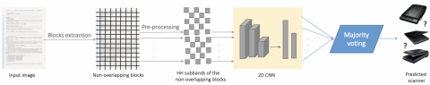
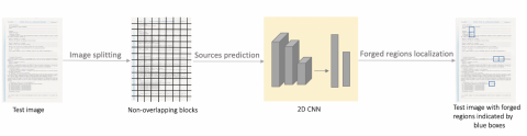
The architecture of our system is depicted in Figure 1. As can be seen, it first cuts the image into non-overlapping blocks. This is an important step in order to obtain enough data for the training process and to avoid memory saturation. Then, these blocks are wavelet transformed and their HH wavelet subbands are used as input of a CNN. Our choice in using this information as CNN input data relies on one of our solution [12] with advanced performance compared to the state of art. This one extracts manually-crafted features (scale and form) in the wavelet domain; features that have been designed to capture the differences between HH DWT coefficient distributions (a generalized Gaussian distribution) of images scanned with different scanners and which have the interest to be less sensitive to the image content. Hence, by feeding CNN with HH subbands coefficients, we expect i) to be able to remove the scanned document content that is not relevant for SSI and, ii) that deep learning will be able to extract the noise mixture that is unique to one scanner.
In this work, we opted for the stationary wavelet transform (SWT) [30] rather than for the traditional DWT due to its better performance for image denoising [31]. Also, SWT avoids coefficient decimation, a property of interest for small images.
The final decision about the source scanner relies on a majority voting considering CNN responses for all image blocks. We come back to the details and the purpose of each of these steps in the sequel.
2.1 Pre-processing: Wavelet decomposition
Wavelet transform (WT) has been successfully applied in a wide variety of scientific fields. In our previous work [12], we explored the DWT transform to: i) suppress block content information so as to better extract the flatbed scanner mixture noise; ii) reduce the dimensions of the data to process. Whereas, in the current work, we rather use SWT, an extension of the traditional DWT, thus neglecting the downsampling step. Indeed, the SWT performs better in image denoising and edge detection and its coefficients remain the same when the image is shifted. An illustration of the DWT and the SWT decompositions is shown in Figure 2, where h1, g1, h2, g2 are the low-pass and high pass wavelet analysis filters. Each decomposition consists in passing the image I through a wavelet filter bank to get approximations coefficients and details coefficients. In the following, the wavelet transforms are performed with the Symlet4 wavelet filter based on the results presented by Rabah et al. [12].
For one decomposition level and for an image of RxC pixels, a dyadic SWT transform produces four subbands of RxC coefficients denoted by LL (Low- Low), LH (Low- High), HL (High-Low), and HH (High- High). As an input to our system, only the HH subband is exploited since it is the one that contains most of the scanner noise [12]. We will see in the experimental section that this pre-processing step is of importance in order to obtain valuable classification results.
Figure 1. Global architecture of our system
Figure 2. (a) DWT decomposition (b) SWT decomposition
2.2 CNN architecture
A key way to achieve high accuracy rate is to design a CNN that is adapted to the identification system desired. The choice of the architecture configuration typically depends on how well the model performs to achieve the highest accuracy and the lowest loss. Figure 3 illustrates our CNN architecture. First, to avoid increasing the number of weights/ parameters of the network, we proposed a shallow CNN with only one convolutional layer. A second main reason of not going deeper is to be able to train the network using considerably less training data. When a coefficient subband enters the network, it goes through this convolutional layer that convolves the input image with 32 kernels of size 3x3 where the kernel stride is by default set to 1. It is followed by the non-linear activation function ReLu to make our network sparse and help the training to quickly converge. The max-pooling operator of window size 2x2 is by next applied in order to reduce the spatial dimension of the input. These pieces of information are the inputs of two fully connected layers of 512 and N neurons, respectively, preceded by a dropout layer with a probability of 0.5 to prevent over-fitting. The layer located at the very end of our network accompanied by the sigmoid activation function plays the role of a classifier which make the source prediction of the input image.
Figure 3. The network structure of the proposed CNN. The numbers below each colored figure are its dimensions
Notice that the N nodes represent the likelihood of the image to be acquired by each scanner, where N is the number of scanners. We will have 8 nodes, one for each scanner. Table 1 sums up the hyper-parameters of our network.
Table 1. Structure of the proposed CNN
|
Layer |
Name |
Size |
|
1 |
Convolution-ReLu |
32 filters of size 3x3 |
|
2 |
Max-Pooling |
2x2 |
|
3 |
Dropout 50% |
- |
|
4 |
FullConnected-ReLu |
512 |
|
5 |
FullConnected-Sigmoid |
N |
After having classified all the blocks of an image under observation, majority voting is adopted in order to take the final decision about the specific scanner that has acquired it. It is calculated as follows:
$\begin{aligned} \mathrm{M}(\mathrm{Q})=\mathrm{k} \text { if occ }(\mathrm{k}) &=\max _{j=1 . n}(\operatorname{occ}(j)) \\ 1 & \leq \mathrm{k} \leq \mathrm{N} \end{aligned}$ (1)
where, Q is the questioned image, k is a scanner among the N scanners available and occ is the occurrence number of a class j with j=1…N defined by:
$\operatorname{occ}(j)=\sum_{j=1}^{M}\left(P_{i}=j\right)$ (2)
where, Pi is the predicted class (i.e. the source scanner) of the ith block of Q and M is the total number of blocks.
In other terms, the scanner the mostly predicted is identified as the source scanner of Q.
To validate the proposed SSI method, several neural network schemes are discussed and compared. Experiments were performed using a dataset of images of different content acquired with 8 commonly-used flatbed scanners (see Table 2). In Table 2, CCD and CIS stand for Charge-Coupled Device and Contact Image Sensors, respectively. Scanners using CCD technology are thicker and cheaper than the ones using CIS. Moreover, they differ in their optical design [32]. The image dataset corresponds to 54 documents of different types (forms, certificates, contracts, records...) of various content (text, figures, stamps...), which were printed on A4 paper with the same printer and then scanned at the same resolution (300dpi) with each scanner. Scanned documents are stored in the TIFF format.
Table 2. Image sources used in our experiments
|
Scanner Id |
Brand |
Model |
Sensor type |
Native resolution |
|
S1 |
Canon |
Lide 120 |
CIS |
2400´4800 |
|
S2 |
Canon |
Lide 220 |
CIS |
4800´4800 |
|
S3 |
Canon |
CanonScan 9000F |
CCD |
4800´4800 |
|
S4 |
Epson |
Perfection V39 |
CIS |
4800 ´4800 |
|
S5 |
Epson |
Perfection V370 -1 |
CCD |
4800´9600 |
|
S6 |
Epson |
Perfection V370 -2 |
CCD |
4800´9600 |
|
S7 |
Epson |
Perfection V550 |
CCD |
6400´9600 |
|
S8 |
HP |
Scanjet Pro 2500 F1 |
CIS |
1200´1200 |
Each of the following schemes has been implemented in Python using Keras deep learning library on a ZOTAC GeForce RTX 2070 SUPER AMP EXTREME GPU with 32 GB of RAM. The RMSprop optimizer [33] was used. The learning rate was set to 10-6 and the training batch size to 32 images. The final training period consists of 49 epochs which provide the smallest loss on validation blocks.
For each CNN model, we randomly selected 40% of the images for the training, 20% for the validation and 40% for the testing. During training, K-fold cross-validation technique [34] is applied to guarantee generalization. In this study, K is set to 5.
3.1 Classification results for the proposed scheme
To train our network, all images from our dataset were split into non-overlapping blocks of size 256x256 pixels. These sub-images are annotated with their corresponding scanner candidate. Thus, in total, we have approximately 48000 scanned sub-images with different varieties of image details.
As stated in Section 2.1, in order to make our system less sensitive to the image content and that it only learns scanner fingerprints, SWT is applied on these samples giving access to HH subbands next used as CNN input.
To test the effectiveness of the proposed neural network in distinguishing scanners, we have carried out a series of experiments. The main purpose of the first experiment is to evaluate the performance of our method when it works on single image blocks, that is to say deciding on the source scanner of a document from one block, only. A decent testing accuracy of 99.31% is obtained. We repeat the same experiments using the DWT instead of the SWT and a decrease in the classification accuracy by 2.31% is observed as shown in Table 3.
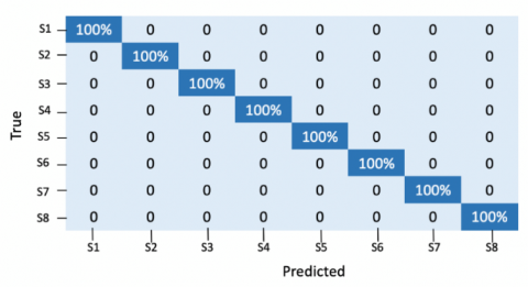
Then, after demonstrating the good performance of our scheme only on a single block, we evaluated the entire pipeline, i.e., CNN along with majority voting based on the decisions obtained from all image blocks. The confusion matrix presented in Figure 4 for classifying full images has an average classification accuracy of 100% using the same dataset which is expected as the majority voting mechanism used in our system would definitely increase the accuracy.
To further evaluate the reliability of our scheme, we propose to use another image test set. 90 new documents were scanned, leading thus to 720 new images next classified with our network. As previously, we obtained 100% of accuracy.
Table 3. Average classification accuracy for non-overlapping blocks and full images for different model architectures
|
|
Accuracy |
|
|
Block level |
Image level |
|
|
AlexNet [35] |
94.69% |
97.5% |
|
GoogleNet [36] |
90.64% |
96.66% |
|
Proposed-DWT |
97% |
100% |
|
Proposed-SWT |
99.31% |
100% |
Figure 4. Confusion matrix for full images using proposed method
In the second experiment, we investigated the impact of the number of convolutional layers on the performance of our scheme. Figure 5 shows that the dynamics of the model with 1, 2, and 3 layers are pretty similar. But the model converges more rapidly with only one convolutional layer, learning thus the problem more quickly.
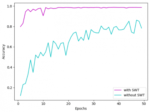
The third experiment evaluates the efficiency of feeding CNN with the HH subband of each block rather than with the block pixel, directly. As can be seen in Figure 6, better performance is achieved compared to the classification without this pre-processing step. This demonstrates the important role of this step. This result shows that it is more appropriate to extract features in the transformed domain than in the spatial domain for SSI.
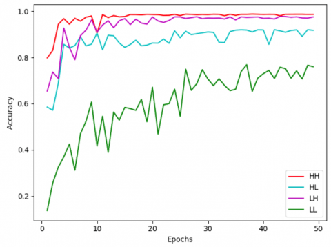
It is interesting to note that scanners embed vertical and horizontal artifacts that can be found in the HL and LH sub-bands. So, an alternative is to use these subbands for SSI. Comparison performance is given in Figure 7. The HH sub-band provides better accuracy results. The LL sub-band is also considered to confirm its non-adaptation to solve SSI problems.
Another important parameter that is crucial when analyzing the performance of the proposed CNN is the choice of the color channels.
Figure 8 shows that a combination of all color channels dramatically improves forecasting accuracy.
Figure 5. Effect of adding convolutional layers to the network
Figure 6. Effect of the pre-processing step on the classification accuracy
Figure 7. Effect of the subband choice on the classification accuracy
Figure 8. Effect of color channels on the performance accuracy
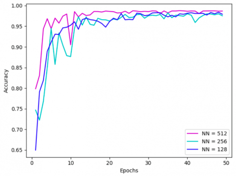
Figure 9. Effect of the number of nodes in the first fully-connected layer
Unlike the above discussed parameters, the effect of the number of nodes NN in the first fully-connected layer is rather neglectable. Yet, the best accuracy is achieved when NN = 512. Such observation, depicted in Figure 9, is likely because higher NN leads to richer representation of the data and, therefore, more accurate predictions. Nevertheless, even with NN = 128 nodes, the neural network yielded great accuracy when compared to more complex models.
3.2 Classification results for different block sizes
The block size is one of the most important parameters of our proposal with an impact on its classification accuracy. Thus, another experiment was carried out in order to show the effect of the block size. Experiments were carried for both DWT and SWT for 2 different block sizes. In Figure 10, we observe the effect of the wavelet transform and the number of samples used for training on the performance of the designed CNN. For the SWT 128 (see Figure 10), our model shows a relatively steady trend, whereas the other models show that the accuracy gradually increases with the increment of the number of training images. This demonstrates that the performance of our model is independent of the size of the training data, whereas an optimum number of training samples has to be selected for other models to attain a high accuracy.
It can be also observed that using the DWT decreases the forecasting accuracy significantly for smaller blocks. These results confirm that the SWT is more suitable than DWT for SSI based on neural networks due to its up-scaling property which likely preserves more information about the scanning noise.
Figure 10. Effect of training size on testing accuracy for multiple block sizes
3.3 Comparison assessments
A comparison of the current method with respect to all the SSI methods in literature is well beyond the scope of the paper since most of them require specific testing image types and/or additional requirements. Therefore, to assess the superiority of our proposal, we propose to compare it with the KLD-based method we proposed by Rabah et al. [12]; a method that has demonstrated better behavior than other recent approaches. Let us recall that Rabah et al. [12] extracts hand-designed features in the wavelet domain. We have also implemented the CNN based method of Shao and Delp [29]. Table 4 shows the various methods and their respective accuracies. As can be seen, our method outperforms the state-of-art methods by obtaining an overall accuracy of 100%. However, Shao and Delp’s method [29] failed to correctly identify most of the scanners. This can be explained by the absence of a pre-processing denoising step which, as shown previously, is necessary to remove the image content. Note that the classification accuracy degrades also in the study [12] along with the increase of the number of scanners to discriminate.
Table 4. Comparison between our proposed method [12, 29]
|
Method |
Accuracy |
|
Shao et al. [29] |
41.10% |
|
KLD-method [12] |
69.23% |
|
Proposed |
100% |
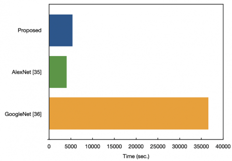
To compare with common CNN, we trained AlexNet [35] and GoogleNet [36] on our image data set, using the same pre-processing strategy. We obtained an accuracy of 94.69% and 90.64% at block level and 97.5% and 96.66% at full image level for AlexNet and GoogleNet, respectively, as reported in Table 3. We further compare the time complexity of each network. Based on the results shown in Figure 11, AlexNet requires the shortest training time but performs the worst in term of classification accuracy. We reported 5227.77s, 4026.55s, and 36607.06s as average training time for our CNN, Alexnet and GoogleNet respectively. Compared to the performance of our scheme, one can conclude that much better performance are achieved with a small, less time-consuming and compact CNN configuration of only one convolutional layer.
Figure 11. Average training time for different CNNs
Figure 12. Forgery detection scheme
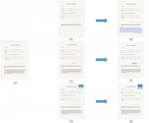
Figure 13. Test case. (a) Original. ((b), (c), and (d)) Tampered. ((e), (f), and (g)) Tampered region detected
3.4 Extension to forgery detection
Image forgery detection techniques [37] are required in many fields for protecting copyright and preventing malicious alteration or falsification of digital documents.
There exist several classes of tampering attacks, the most considered ones being copy-move and splicing forgeries.
Copy-move forgeries consist in cloning a part of an image and pasting it in a different location. While, in splicing, the pasted block comes from a different image.
To address these issues, we propose to use our SSI solution to approximately localize the tampered regions in fake document images independently of the shape of the forged area.
The idea is to identify the scanner at the origin of a questioned image, divide it into non-overlapping blocks and then to find blocks that are predicted to be scanned with a different scanner. These incorrectly identified blocks, marked by bounding blue boxes, indicates suspicious copied area. The proposed forgery detection scheme is illustrated in Figure 12.
We select a block of size 64 so as to get a more precise detection. An example is illustrated in Figure 13. The left image represents the original image. In the middle, 3 cases of forgeries are given:
It is immediate to observe in the remaining images that the altered regions are marked with blue rectangles with a relatively high precision. Therefore, the investigated solution is able to effectively alleviate the problem of some forgeries detection.
In this paper, we proposed a novel approach that exploits the scanner noise located in the wavelet HH subband while simultaneously benefiting of the capacity of CNN to automatically extract useful features from this subband.
Classification results demonstrate that our CNN offers superior performance than recent scanner identification techniques even under the condition of limited training samples. Another result of our scheme is that it is able to identify the source scanner even from small blocks of the image. This is a promising prospect for forensics applications particularly when only a part of the investigated image is available such as forgery detection. The proposed method succeeded to detect digitally forged regions given only the forged image.
Future works will focus on expanding our network to take into consideration a greater number of scanners as well as proposing a more reliable tampering localization.
This work was financially supported by the "PHC Utique" program of the French Ministry of Foreign Affairs and Ministry of higher education and research and the Tunisian Ministry of higher education and scientific research in the CMCU project number 17G1406.
[1] Sailaja, R., Rupa, C., Chakravarthy, A.S.N. (2017). Robust and indiscernible multimedia watermarking using light weight mutational methodology. Traitement du Signal, 34(1-2): 45-55. https://doi.org/10.3166/TS.34.45-55
[2] Narayana, V.L., Gopi, A.P. (2017). Visual cryptography for gray scale images with enhanced security mechanisms. Traitement du Signal, 34(3-4): 197-208. https://doi.org/10.3166/TS.34.197-208
[3] Duan, Y., Bouslimi, D., Yang, G., Shu, H., Coatrieux, G. (2016). Computed tomography image origin identification based on original sensor pattern noise and 3-D image reconstruction algorithm footprints. IEEE Journal of Biomedical and Health Informatics, 21(4): 1039-1048. https://doi.org/10.1109/JBHI.2016.2575398
[4] Gloe, T., Franz, E., Winkler, A. (2007). Forensics for flatbed scanners. In Security, Steganography, and Watermarking of Multimedia Contents IX, 6505: 65051I. https://doi.org/10.1117/12.704165
[5] Gou, H., Swaminathan, A., Wu, M. (2007). Robust scanner identification based on noise features. In Security, Steganography, and Watermarking of Multimedia Contents IX, 6505: 65050S. https://doi.org/10.1117/12.704688
[6] Khanna, N., Mikkilineni, A.K., Chiu, G.T., Allebach, J.P., Delp, E.J. (2007). Scanner identification using sensor pattern noise. In Security, Steganography, and Watermarking of Multimedia Contents IX, 6505: 65051K. https://doi.org/10.1117/12.705837
[7] Gou, H., Swaminathan, A., Wu, M. (2009). Intrinsic sensor noise features for forensic analysis on scanners and scanned images. IEEE Transactions on Information Forensics and Security, 4(3): 476-491. https://doi.org/10.1109/TIFS.2009.2026458
[8] Khanna, N., Mikkilineni, A.K., Delp, E.J. (2009). Scanner identification using feature-based processing and analysis. IEEE Transactions on Information Forensics and Security, 4(1): 123-139. https://doi.org/10.1109/TIFS.2008.2009604
[9] Rabah, C.B., Coatrieux, G., Abdelfattah, R. (2019). Semi-blind source scanner identification. In 2019 International Conference on Internet of Things, Embedded Systems and Communications (IINTEC), pp. 220-225. https://doi.org/10.1109/IINTEC48298.2019.9112109
[10] Choi, C.H., Lee, M.J., Lee, H.K. (2010). Scanner identification using spectral noise in the frequency domain. 2010 IEEE International Conference on Image Processing, Hong Kong, pp. 2121-2124. https://doi.org/10.1109/ICIP.2010.5652108
[11] Rabah, C.B., Abdallah, W.B., Abdelfattah, R., Bouslimi, D., Coatrieux, G. (2017). Identification de l’origine d’un document numerise sur la base d’une empreinte de scanner dans le domaine des ondelettes. Computer Electronics Security Applications Rendez-vous (C&ESAR).
[12] Rabah, C.B., Coatrieux, G., Abdelfattah, R. (2018). Scanner model identification of official documents using noise parameters estimation in the wavelet domain. In International Conference on Advanced Concepts for Intelligent Vision Systems, 111852: 598-608. https://doi.org/10.1007/978-3-030-01449-0_50
[13] Khanna, N., Delp, E.J. (2009). Source scanner identification for scanned documents. 2009 First IEEE International Workshop on Information Forensics and Security (WIFS), London, pp. 166-170. https://doi.org/10.1109/WIFS.2009.5386462
[14] Khanna, N., Delp, E.J. (2010). Intrinsic signatures for scanned documents forensics: Effect of font shape and size. Proceedings of 2010 IEEE International Symposium on Circuits and Systems, Paris, pp. 3060-3063. https://doi.org/10.1109/ISCAS.2010.5537996
[15] Joshi, S., Gupta, G., Khanna, N. (2017). Source classification using document images from smartphones and flatbed scanners. In National Conference on Computer Vision, Pattern Recognition, Image Processing, and Graphics, 841: 281-292. https://doi.org/10.1007/978-981-13-0020-2_25
[16] Sugawara, S. (2014). Identification of scanner models by comparison of scanned hologram images. Forensic Science International, 241: 69-83. https://doi.org/10.1016/j.forsciint.2014.04.018
[17] Dirik, A.E., Sencar, H.T., Memon, N. (2009). Flatbed scanner identification based on dust and scratches over scanner platen. 2009 IEEE International Conference on Acoustics, Speech and Signal Processing, Taipei, pp. 1385-1388. https://doi.org/10.1109/ICASSP.2009.4959851
[18] Elsharkawy, Z.F., Abdelwahab, S.A.S., Dessouky, M.I., Elaraby, S.M., Abd El-Samie, F.E. (2013). C20. Identifying unique flatbed scanner characteristics for matching a scanned image to its source. 2013 30th National Radio Science Conference (NRSC), Cairo, Egypt, pp. 298-305. https://doi.org/10.1109/NRSC.2013.6587928
[19] Mane, D.T., Kulkarni, U.V. (2020). A survey on supervised convolutional neural network and its major applications. In Deep Learning and Neural Networks: Concepts, Methodologies, Tools, and Applications, 1058-1071. https://doi.org/10.4018/978-1-7998-0414-7.ch059
[20] Kim, D.G., Hou, J.U., Lee, H.K. (2019). Learning deep features for source color laser printer identification based on cascaded learning. Neurocomputing, 365: 219-228. https://doi.org/10.1016/j.neucom.2019.07.084
[21] Tsai, M.J., Tao, Y.H., Yuadi, I. (2019). Deep learning for printed document source identification. Signal Processing: Image Communication, 70: 184-198. https://doi.org/10.1016/j.image.2018.09.006
[22] Rafi, A. M., Kamal, U., Hoque, R., Abrar, A., Das, S., Laganière, R., Hasan, M.K. (2019). Application of DenseNet in camera model identification and post-processing detection. In CVPR Workshops, pp. 19-28.
[23] Ding, X., Chen, Y., Tang, Z., Huang, Y. (2019). Camera identification based on domain knowledge-driven deep multi-task learning. IEEE Access, 7: 25878-25890. https://doi.org/10.1109/ACCESS.2019.2897360
[24] Zou, Z., Liu, Y., Zhang, W., Chen, Y. (2019). Camera model identification based on residual extraction module and SqueezeNet. In Proceedings of the 2nd International Conference on Big Data Technologies, pp. 211-215. https://doi.org/10.1145/3358528
[25] Yang, P., Ni, R., Zhao, Y., Zhao, W. (2019). Source camera identification based on content-adaptive fusion residual networks. Pattern Recognition Letters, 119: 195-204. https://doi.org/10.1016/j.patrec.2017.10.016
[26] Al Banna, M.H., Haider, M.A., Al Nahian, M.J., Islam, M.M., Taher, K.A., Kaiser, M.S. (2019). Camera model identification using deep CNN and transfer learning approach. In 2019 International Conference on Robotics, Electrical and Signal Processing Techniques (ICREST), pp. 626-630. https://doi.org/10.1109/ICREST.2019.8644194
[27] Rafi, A.M., Tonmoy, T.I., Kamal, U., Hoque, R., Hasan, M. (2019). RemNet: Remnant convolutional neural network for camera model identification. Neural Computing and Applications, 1-16.
[28] Freire-Obregón, D., Narducci, F., Barra, S., Castrillón-Santana, M. (2019). Deep learning for source camera identification on mobile devices. Pattern Recognition Letters, 126: 86-91. https://doi.org/10.1016/j.patrec.2018.01.005
[29] Shao, R., Delp, E.J. (2020). Forensic scanner identification using machine learning. 2020 IEEE Southwest Symposium on Image Analysis and Interpretation (SSIAI), Albuquerque, NM, USA, pp. 1-4. https://doi.org/10.1109/SSIAI49293.2020.9094618
[30] Fowler, J.E. (2005). The redundant discrete wavelet transform and additive noise. IEEE Signal Processing Letters, 12(9): 629-632. https://doi.org/10.1109/LSP.2005.853048
[31] Kumar, R., Patel, P. (2012). Signal denoising with interval dependent thresholding using DWT and SWT. International Journal of Innovative Technology and Exploring Engineering (IJITEE), 1(6): 47-50.
[32] Rabah, C.B., Coatrieux, G., Abdelfattah, R. (2020). The supatlantique scanned documents database for digital image forensics purposes. 2020 IEEE International Conference on Image Processing (ICIP), Abu Dhabi, United Arab Emirates, pp. 2096-2100. https://doi.org/10.1109/ICIP40778.2020.9190665
[33] Rodriguez, J.D., Perez, A., Lozano, J.A. (2009). Sensitivity analysis of k-fold cross validation in prediction error estimation. IEEE Transactions on Pattern Analysis and Machine Intelligence, 32(3): 569-575. https://doi.org/10.1109/TPAMI.2009.187
[34] Krizhevsky, A., Sutskever, I., Hinton, G.E. (2017). Imagenet classification with deep convolutional neural networks. Communications of the ACM, 60(6): 84-90. https://doi.org/10.1145/3065386
[35] Szegedy, C., Liu, W., Jia, Y., Sermanet, P., Reed, S., Anguelov, D., Rabinovich, A. (2015). Going deeper with convolutions. 2015 IEEE Conference on Computer Vision and Pattern Recognition (CVPR), Boston, MA, pp. 1-9. https://doi.org/10.1109/CVPR.2015.7298594
[36] Tieleman, T., Hinton, G. (2012). Divide the gradient by a running average of its recent magnitude. COURSERA Neural Netw. Mach. Learn, 6: 26-31.
[37] Barad, Z.J., Goswami, M.M. (2020). Image forgery detection using deep learning: A survey. In 2020 6th International Conference on Advanced Computing and Communication Systems (ICACCS), pp. 571-576.