Behnam Asghari Beirami* | Mehdi Mokhtarzade
© 2020 IIETA. This article is published by IIETA and is licensed under the CC BY 4.0 license (http://creativecommons.org/licenses/by/4.0/).
OPEN ACCESS
In this paper, a novel feature extraction technique called SuperMNF is proposed, which is an extension of the minimum noise fraction (MNF) transformation. In SuperMNF, each superpixel has its own transformation matrix and MNF transformation is performed on each superpixel individually. The basic idea behind the SuperMNF is that each superpixel contains its specific signal and noise covariance matrices which are different from the adjacent superpixels. The extracted features, owning spatial-spectral content and provided in the lower dimension, are classified by maximum likelihood classifier and support vector machines. Experiments that are conducted on two real hyperspectral images, named Indian Pines and Pavia University, demonstrate the efficiency of SuperMNF since it yielded more promising results than some other feature extraction methods (MNF, PCA, SuperPCA, KPCA, and MMP).
minimum noise fraction, superpixel, feature extraction, hyperspectral classification, SuperMNF
The high dimensionality of hyperspectral data and the limited size of training samples make the supervised classification of hyperspectral images challenging. The so-called Hughes phenomenon states that this high dimensionality will not necessarily lead to better performance of classification algorithms. To alleviate these challenges, commonly, dimensionality reduction (DR) techniques are used that are divided into two major groups; feature selection and feature extraction. In feature extraction (FE) methods that are the subject of this paper, original spectral bands are transformed into a new low dimensional space. FE methods are divided into supervised or unsupervised techniques based on whether the training samples are used.
Linear discriminant analysis (LDA) [1], non-parametric weighted feature extraction (NWFE) [2], clustering-based feature extraction (CBFE) [3], and local fisher discriminant analysis (LFDA) [4] are perhaps the most used supervised methods. Generally, the performance of supervised methods depends on the quality and numbers of training samples. On the other hand, unsupervised methods do not require any training samples.
Principal components analysis (PCA) is a simple unsupervised FE method that is used in many fields of remote sensing image analysis. PCA transforms the original spectral feature of HSI into a new space in which the extracted features are sorted based on their variances, and the most informative features lie on the first few components. In recent years, some spatial-spectral classification methods are proposed in literature based on the PCA technique. Residual deep PCA (RDPCA) that are proposed to combine Deep PCA with residual-based multi-scale feature extraction for HSI classification [5]. Gabor based random patches network is proposed for classification of hyperspectral image based on the idea of PCANet to extract the deep features [6]. The minimum noise fraction (MNF) method incorporates the noise covariance matrix in the process of FE, and final features are sorted based on the signal-to-noise ratio (SNR) [7, 8]. Different version of PCA method named, PCA and SPCA (Segmented-PCA), SSPCA (Spectrally SegmentedPCA), FPCA (Folded-PCA), KPCA (Kernel-PCA) and KECA (kernel Entropy Component Analysis) are compared with MNF transform [9] and final results shows the superiority of MNF transform in classification accuracy.
In addition to mentioned information-based methods some other FE methods based on graph learning and manifold-learning methods are proposed in literature. Local neighborhood structure preserving embedding (LNSPE) method is newly proposed method [10] the branch of graph-based method which uses the scatter information and the dual graph structure to extract the new features. In the branch of manifold-based methods, locality preserving projection (LPP) [11] and its new version (TwoSP) [12] are proposed for classification of hyperspectral images. In addition to mentioned unsupervised methods, some semi-supervised methods are proposed in the literature, such as maximum margin projection (MMP) that utilizes both labelled and unlabelled samples [13].
In contrast to the above-mentioned transformation-based methods in which whole pixels of HSI are transformed into new feature space via one transformation matrix, some pixel-based unsupervised FE methods are proposed in the literature. As an example, the rational function curve fitting feature extraction method (RFCF) fitted a rational function to the spectral signature curve of each pixel, and its coefficients are regarded as the new extracted features [14]. Another example is spectral segmentation and integration (SSI) method based on PSO optimization [15]. In this method each spectral curve is spilited to segments based on PSO optimization and in each segment weighted mean operator is used to extract the new spectral feature.
As proved in literature, incorporating the spatial information can improve the HSI classification accuracy. Random patches network (RPNet) that is proposed by Xu et al. [16] is the multilayer deep model based on PCA transform for extracting the spatial-spectral HSI features. A novel hybrid neural network (HNN) for hyperspectral image classification method is proposed by Li et al. [17] that use a multi-branch architecture, deconvolution structure, batch normalization (BN) technique, and parametric rectified linear units (PReLU) to extract deep hyperspectral image features.
Generally, the transformation matrices of traditional FE methods (such as PCA and MNF) is computed based on the statistics that are estimated from the entire image, so they cannot obtain the local characteristics of pixels in HSI. Recently some spatial-spectral dimensionality reduction methods such as Superpixel-based PCA (SuperPCA) proposed to address this issue [18]. Based on SuperPCA, it is proved that the transformation matrix of the PCA has a local characteristic. The basic idea behind SuperPCA is that different superpixels need different PCA transformation matrices. This concept is extended further [19] named band grouping SuperPCA (BG_SuperPCA) in which SuperPCA is used to extract the new features in each correlated band group, separately. A new method is proposed by Zhang et al. [20] in which a multiscale classifier system is designed based on Superpixel-based Kernel PCA. Another classification method [21] is proposed based on the superpixel pattern features that are extracted by PCA and kernel extreme learning machine (KELM). As one can see, superpixel-based dimensionality reduction of hyperspectral images is a hot topic in literature.
Although SuperPCA outperforms the traditional PCA, it just attempts to provide local new features with maximum dispersion while the noise content is not taken into consideration. In this paper, we put forward the question that “Does it make sense to implement the traditional MNF on individual superpixels and how effective it could be in comparison to the traditional MNF and the SuperPCA methods?”. In other words, in this study, a novel method called Superpixel-based MNF (SuperMNF) is proposed in which extracted features of each superpixel are sorted based on SNR rather than variance (SuperPCA).
In the next section, the concept of MNF transformation and entropy rate superpixel (ERS) generation method are reviewed as the background. It is followed by the introduction of SuperMNF. The next section deals with the experimental results, and the paper ends with the conclusions.
This section reviews the concept of MNF transformation and the entropy rate superpixel (ERS) generation method.
2.1 MNF transform
Given W∈RM×d as the transformation matrix, and X∈RM×N as the original spectral data matrix in which, M is the number of HSI bands, N is the number of HSI pixels, and d is the new dimension size of data. Extracted features matrix of MNF Y∈Rd×N can be shown as (1):
$Y=W^{T} X$ (1)
X as the original data matrix, herein an HSI, can be regarded as a signal part S and an additive noise part N (2):
X=S+N (2)
Therefore, the covariance matrix of X is the summation of signal and noise covariance matrices as follows:
$\Sigma_{X}=\Sigma_{S}+\Sigma_{N}$ (3)
where, ∑S is the covariance of signal and ∑N is the covariance of noise. MNF, as a linear transformation, aims to provide new features (Y) in a way to be sorted according to their SNR. W can be obtained by solving the following problem [22]:
$\operatorname{argmax}_{W} \frac{W^{T} \sum_{X} W}{W^{T} \sum_{N} W}-1$ (4)
For that purpose, W must be made up of the eigenvectors associated with sorted eigenvalues of $\sum_{N}^{-1} \sum_{X}$. To estimate the covariance of noise ∑N, minimum/maximum auto-correlation factor (MAF) [8] is used in this paper. This method consists of two stages. At the first stage, noise image is produced from each band of HSI based on formula (5):
Noise image $=x_{(i, j, k)}-x_{(i+\Delta 1, j+\Delta 2, k)}$ (5)
In (5) x(i,j,k) represents the kth spectral band of HSI image in which the row and column of pixels are shown by i and j, respectively. ∆1 and ∆2 are the spatial lags along each coordinate axes which are usually assumed to 1. After that, covariance of noise ∑N is estimated based on (6) [8]:
$\Sigma_{N}=0.5 \operatorname{cov}($Noise image$)$ (6)
2.2 Entropy rate superpixel segmentation (ERS)
ERS is the efficient graph-based method for implementing the superpixel segmentation. In this method, graph G= (V, E) is considered in which V and E represent the pixels and pairwise similarities, respectively. ERS aims at selecting a subset of edges A (A⊆ E) in a way so as to yield graph G= (V, A) containing the K sub-graphs. The objective function of ERS is as follows [23]:
$\max _{A} H(A)+\tau B(A)$ s.t. $A \subseteq E$ (7)
where, H(A) named entropy rate, B(A) is balancing term and $\tau$ is the non-negative weight of balancing term. Entropy rate H(A) and balancing term B(A) are considered to create compact and homogeneous superpixels with similar sizes. Greedy algorithm is used to solve the (7). Given Q as the 1-band superpixels are obtained based on formula (8) [18]:
$Q=\cup_{n=1}^{n} K_{n}$ s.t. $K_{i} \cap K_{j}=\emptyset$ for each $i \neq j$ (8)
where, Kn representing nth superpixel.
The main critique of traditional MNF is that it considers global noise and signal covariance matrices for the whole image to estimate the transformation matrix W, while these matrices have local characteristics. In Figure 1, the global noise and signal covariance matrices that are estimated from entire image are shown beside two local ones, each of which estimated for a specific superpixel.
Figure 1. ∑X and ∑N of -a,b) the whole image- c,d) a specific super pixel- e,f) another superpixel
Figure 2. Flowchart of SuperMNF feature extraction method
The Figure 1 confirms the idea of SuperPCA states that signal covariance matrices (∑X) have local characteristics (Figure 1. b, d, f). As the new result this study found that noise covariance matrices have the local characteristics (Figure 1. a, c, e) same as signal covariance matrices, since there are significant differences between the matrices of different superpixels as well as the whole image. In this study, the SuperMNF method is proposed in that the transformation matrix (W) is computed for each superpixel individually. The resultant MNF transformation is also confined to those pixels of the corresponding superpixel.
Figure 2 shows the flowchart of SuperMNF. According to Figure 2 SuperMNF method has the seven stages as below:
Unlike the MNF transform in that ∑X and ∑N are computed based on the entire image, in SuperMNF Methods these matrices are estimated in each superpixel separately. Therefore, in SuperMNF estimated covariance matrices have local characteristics in that the information of a specific superpixel has no impact on another superpixel.
4.1 Data sets
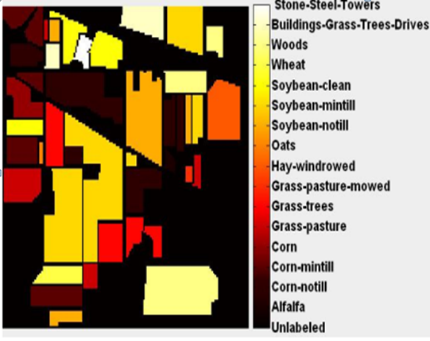
Indian Pines: Indian Pines scene is collected by AVIRIS airborne hyperspectral sensor in 224 spectral bands. It has 145×145 pixels with a 20-meter spatial resolution. After discarding the noisy and water absorption bands, the remaining 204 spectral bands are used in analyses. 16 agricultural classes are recognized in this image based on ground truth. Figure 3 shows the color composite of Indian Pines followed by its ground truth image [24].
a. colour composite image
b. ground truth image
Figure 3. Indian Pines data set
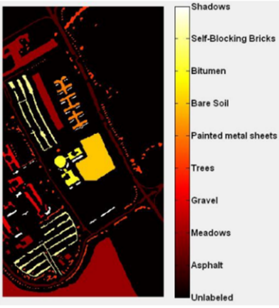
a. colour composite image
b. ground truth image
Figure 4. Pavia University data set
Pavia University: Pavia University hyperspectral image is gathered by ROSIS airborne hyperspectral sensor in 115 spectral bands. It has 610×340 pixels with a 1.3-meter spatial resolution from an urban area. After removing the 12 noisy and water absorption bands, the remaining 103 bands are used in analyses. Figure 4 shows the color composite of Pavia University, followed by its ground truth image.
4.2 Parameters analysis
The number of superpixels is an important factor of SuperMNF, so in the first experiment, we study the effect of this parameter in the performance of SuperMNF. Different numbers of superpixels have been examined in this experiment. In each situation with the specific number of the superpixel, 1 to 10 extracted features of SuperMNF are fed to maximum likelihood classifier (MLC), and the maximum of the overall accuracies in each case is reported in Figure 5 for both data sets.
a
b
Figure 5. Profiles of the max overall accuracy of SuperMNF features- a) Indian Pines-b) Pavia University
According to Figure 5, the optimum number of superpixel for Indian Pines and Pavia University are 34 and 11, respectively. The optimum number of superpixels is affected by the number, size, and spatial distribution of classes. Indian Pines image contains different crops in rather small spatial sizes and therefore, a higher number of superpixels is required to represent the local distribution of the scene. It should be noted that choosing the large numbers of superpixels may lead to near singular estimation of signal or/and noise covariance matrices (numbers of superpixels above 37 and 12 for Indian pines and Pavia University, respectively). As the rule of thumb, virtual dimensionality (VD) estimation with Harsanyi–Farrand–Chang (HFC) Method [25] can be used to estimate the optimum number of superpixels in SuperMNF method (VD estimation with false alarm of 10-7 are 34 and 11 for Indian Pines and Pavia University, respectively).
4.3 Comparison with some conventional FE methods
To investigate the robustness of proposed method, for both data sets two sizes of training samples (15 and 30 samples in each class for Indian Pines, 15 and 45 samples in each class for Pavia University data set) are randomly chosen from ground truths for training the supervised classifiers, and remainder samples of ground truths are chosen as test samples for evaluating the classification accuracy.
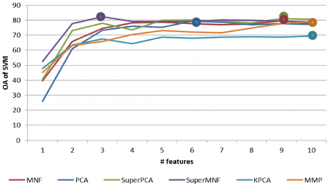
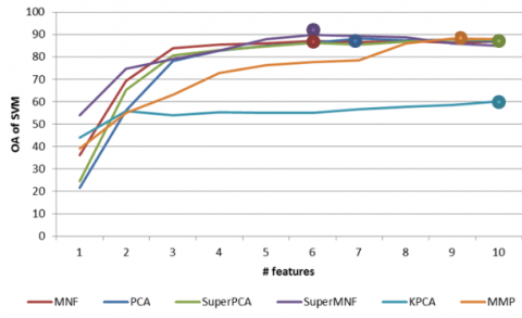
By considering the optimum numbers of superpixels for both data sets from previous sub-section (4.2), different numbers of extracted features (from 1 to 10) of SuperMNF and other five FE methods (traditional MNF, PCA, KPCA, SuperPCA, and MMP) are classified via maximum likelihood and support vector machines (SVM). Parameters of SVM with radial basis functions are set via cross-validation.
The obtained results of overall accuracies are shown in Figure 6 for Indian Pines and Pavia University, respectively. As a result, SuperMNF is superior in comparison to other FE methods. This superiority can be traced to the ability of SuperMNF to extract the local features that are derived from local transformation matrices.
In general, based on the experiments it can be concluded that the SuperPCA is the most important competitor method as it has the nearer results to SuperMNF than other methods. The highest difference between the results of SuperPCA and SuperMNF is achieved in the Pavia University data set when we used the MLC as the classifier and 15 training samples. From this result, we can conclude that the proposed method can be successfully used in the challenging urban areas even when very few training samples are available for the classification of HSI.
Achieved highest overall accuracies (OA) and highest average accuracies (AA) of each feature extraction method for both data sets are shown in Table 1. Due to the high dimensionality of original data and few numbers of training samples, MLC failed to estimate its parameter that is shown by “NAN” in this Table 1. Based on Table 1, it is clear that the SuperMNF method is superior against all other FE methods in the term of OA and AA accuracy measures. In comparison to SuperPCA, commonly, SuperMNF achieves the highest accuracies in the fewer number of features which can decrease the storage for saving the HSI image. Another important result from Table 1 is that the mean accuracy of classification in the SuperMNF method in Indian pines (agricultural areas) is higher than the Pavia University (urban areas). In other words, it seems that the proposed SuperMNF has a better performance in agricultural areas than urban areas.
Table 1. Classification accuracies of different FE methods in different data sets maximum OA [maximum AA](# of features)
|
Classifiers |
MLC classifier |
SVM classifier |
|||||||
|
Data sets |
Indian Pines |
Pavia University |
Indian Pines |
Pavia University |
|||||
|
# of training samples |
15 |
30 |
15 |
45 |
15 |
30 |
15 |
45 |
|
|
Methods |
Original Spectral |
NAN |
NAN |
NAN |
NAN |
63.68 [74.5] (200) |
67 [66.27] (200) |
72.93 [82.57] (103) |
85.98 [88.36] (103) |
|
SuperMNF |
89.47 [89.57] (9) |
90.77 [82.17] (9) |
82.12 [86.87] (6) |
89.69 [91.81] (6) |
91.63 [94.4] (8) |
94.13 [84.3] (7) |
82.40 [88.33] (3) |
94.01 [95.5] (5) |
|
|
SuperPCA |
85.68 [89.14] (10) |
86.77 [79.29] (7) |
70.11 [77.23] (6) |
87.61 [89.11] (10) |
89.02 [92.37] (8) |
86.77 [80.49] (7) |
80.99 [87] (9) |
92.89 [94.24] (10) |
|
|
MNF |
67.16 [79.95] (7) |
71.86 [70.51] (8) |
81.34 [84.79] (4) |
87.16 [88.76] (6) |
72.77 [84.45] (8) |
77.16 [74.4] (8) |
79.72 [86.7] (9) |
86.4 [88.71] (9) |
|
|
PCA |
58.4 [65.4] (6) |
59.35 [57.17] (5) |
77.02 [81.61] (7) |
88.22 [88.95] (7) |
56.07 [68.2] (5) |
58.5 [58.3] (5) |
79.41 [85.5] (6) |
87.14 [89.61] (8) |
|
|
KPCA |
54.71 [59.23] (7) |
56.08 [55.09] (10) |
65.90 [78] (8) |
60.10 [78.63] (10) |
52.77 [66.09] (10) |
57.5 [58.83] (10) |
69.36 [78.67] (10) |
75.59 [83.12] (10) |
|
|
MMP |
52.12 [56.88] (7) |
55.52 [52.49] (8) |
78.42 [77.52] (9) |
88.08 [88.2] (9) |
50.69 [62.58] (10) |
56.18 [57.36] (10) |
79.11 [86.6] (10) |
86.22 [87.8] (10) |
|
MLC accuracies of Indian Pines for 15 training samples
SVM accuracies of Indian Pines for 15 training samples
MLC accuracies of Indian Pines for 30 training samples
SVM accuracies of Indian Pines for 30 training samples
MLC accuracies of Pavia University for 15 training samples
SVM accuracies of Pavia University for 15 training samples
MLC accuracies of Pavia University for 45 training samples
SVM accuracies of Pavia University for 45 training samples
Figure 6. Profiles of the overall accuracy of 1 to 10 SuperMNF features against other FE
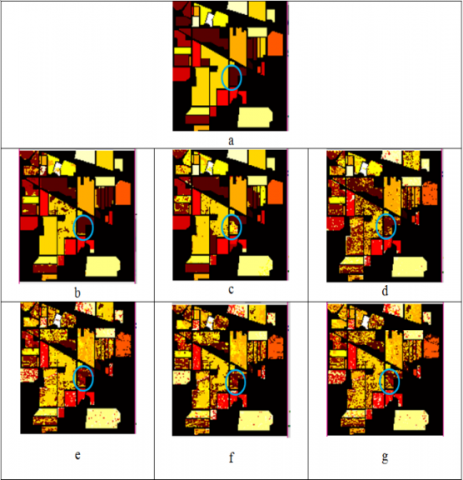
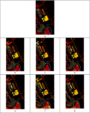
To visually comparison of classification results which are achieved in each method, ground truth and MLC classification maps of each method for the both data set are shown in Figure 7 and Figure 8 when 15 training samples are available. Based on these images, result of best classification method is as near as ground truth in each data set. As can understand from the figures, the SuperMNF method has produced smoother classification maps in comparison to other FE methods.
Figure 7. Indian Pines data set- Classified Maps of MLC in different FE methods- a) Ground truth – b) SuperMNF – c) SuperPCA – d) MNF – e) PCA – f) KPCA – g) MMP
Figure 8. Pavia University data set-Classified Maps of MLC in different FE methods- a) Ground truth – b) SuperMNF – c) SuperPCA – d) MNF – e) PCA – f) KPCA – g) MMP
Table 2. Processing times in second and percent for different FE methods
|
SuperMNF |
SuperPCA |
MNF |
PCA |
KPCA |
MMP |
|
2.5 |
1.17 |
1.11 |
0.5 |
121 |
2.72 |
|
ref |
46.7% |
44.4% |
20% |
4840% |
108.8% |
Table 2 provides the spent processing times at the cores of each FE method in Indian Pines data set. All experiments are implemented in Matlab 2018b with a desktop computer with specifications of Intel(R) Core(TM) i5-6400 CPU and 8.00 GB RAM.
Although the proposed SuperMNF is not superior in computational time aspects, its processing time is still in the competition with many other FE methods. Generally, the MNF method has more steps for extracting new features than PCA. These steps include noise image calculation and noise covariance estimation. As the result in general MNF is slower than PCA so SuperMNF is slower than SuperPCA. From the comparison of SuperMNF and MNF, it can understand that more processing time of SuperMNF is due to the superpixel segmentation stage and estimating the covariance of noise and its inverse in each superpixel.
In this paper, A new extension of classical MNF named SuperMNF is proposed in which local features are extracted by applying the classical MNF to each superpixel, individually. Extracted features are then classified via two classifiers, maximum likelihood (MLC) and support vector machines (SVM). Final classification accuracies results proved the superiority of SuperMNF in comparison to traditional MNF, PCA, KPCA, SuperPCA, and MMP. Based on our experimental results, we can summarize the achievements of paper in the following points:
In the future study, we will design the multiple classifier systems based on multiscale Super MNF is hugely improved.
[1] Prasad, S., Bruce, L.M. (2008). Limitations of principal components analysis for hyperspectral target recognition. IEEE Geoscience and Remote Sensing Letters, 5(4): 625-629. https://doi.org/10.1109/LGRS.2008.2001282
[2] Kuo, B.C., Landgrebe, D.A. (2002). Hyperspectral data classification using nonparametric weighted feature extraction. IEEE International Geoscience and Remote Sensing Symposium, 3: 1428-1430. https://doi.org/10.1109/TGRS.2004.825578
[3] Imani, M., Ghassemian, H. (2013). Band clustering-based feature extraction for classification of hyperspectral images using limited training samples. IEEE Geoscience and Remote Sensing Letters, 11(8): 1325-1329. https://doi.org/10.1109/LGRS.2013.2292892
[4] Li, W., Prasad, S., Fowler, J.E., Bruce, L.M. (2011). Locality-preserving dimensionality reduction and classification for hyperspectral image analysis. IEEE Transactions on Geoscience and Remote Sensing, 50(4): 1185-1198. https://doi.org/10.1109/TGRS.2011.2165957
[5] Ye, M., Ji, C., Chen, H., Lei, L., Lu, H., Qian, Y. (2019). Residual deep PCA-based feature extraction for hyperspectral image classification. Neural Computing and Applications, 32: 1-14. https://doi.org/10.1007/s00521-019-04503-3
[6] Beirami, B.A., Mokhtarzade, M. (2019). Spatial-spectral random patches network for classification of hyperspectral images. Traitement du Signal, 36(5): 399-406. https://doi.org/10.18280/ts.360504
[7] Guan, L.X., Xie W.X., Pei, J.H. (2015). Segmented minimum noise fraction transformation for efficient feature extraction of hyperspectral images. Pattern Recognition, 48(10): 3216-26. https://doi.org//10.1016/j.patcog.2015.04.013
[8] Green, A.A., Berman, M., Switzer, P., Craig, M.D. (1988). A transformation for ordering multispectral data in terms of image quality with implications for noise removal. IEEE Transactions on Geoscience and Remote Sensing, 26(1): 65-74. https://doi.org/10.1109/36.3001
[9] Uddin, M.P., Mamun, M.A., Hossain, M.A. (2020). PCA-based feature reduction for hyperspectral remote sensing image classification. IETE Technical Review, 1-21. https://doi.org/10.1080/02564602.2020.1740615
[10] Shi, G., Huang, H., Wang, L. (2019). Unsupervised dimensionality reduction for hyperspectral imagery via local geometric structure feature learning. IEEE Geoscience and Remote Sensing Letters, 17(8): 1425-1429. https://doi.org/10.1109/LGRS.2019.2944970
[11] He, X., Niyogi, P. (2004). Locality preserving projections. In Advances in Neural Information Processing Systems, 153-160.
[12] Li, X., Zhang, L., You, J. (2018). Hyperspectral image classification based on two-stage subspace projection. Remote Sensing, 10(10): 1565. https://doi.org/10.3390/rs10101565
[13] He, X.F., Deng, C., Han, J. (2007). Learning a maximum margin subspace for image retrieval. IEEE Transactions on Knowledge and Data Engineering, 20(2): 189-201. https://doi.org/10.1109/TKDE.2007.190692
[14] Hosseini, S.A., Ghassemian, H. (2016). Rational function approximation for feature reduction in hyperspectral data. Remote Sensing Letters, 7(2): 101-110. https://doi.org/10.1080/2150704X.2015.1101180
[15] Moghaddam, S.H.A., Mokhtarzade, M., Beirami, B.A. (2020). A feature extraction method based on spectral segmentation and integration of hyperspectral images. International Journal of Applied Earth Observation and Geoinformation, 89: 102097. https://doi.org/10.1016/j.jag.2020.102097
[16] Xu, Y., Du, B., Zhang, F., Zhang, L. (2018). Hyperspectral image classification via a random patches network. ISPRS Journal of Photogrammetry and Remote Sensing, 142: 344-357. https://doi.org/10.1016/j.isprsjprs.2018.05.014
[17] Li, J., Liang, B., Wang, Y. (2020). A hybrid neural network for hyperspectral image classification. Remote Sensing Letters, 11(1): 96-105. https://doi.org/10.1080/2150704X.2019.1686780
[18] Jiang, J., Ma, J., Chen, C., Wang, Z., Cai, Z., Wang, L. (2018). SuperPCA: A superpixelwise PCA approach for unsupervised feature extraction of hyperspectral imagery. IEEE Transactions on Geoscience and Remote Sensing, 56(8): 4581-4593. https://doi.org/10.1109/TGRS.2018.2828029
[19] Beirami, B.A., Mokhtarzade, M. (2020). Band grouping SuperPCA for feature extraction and extended morphological profile production from hyperspectral images. IEEE Geoscience and Remote Sensing Letters, 17(11): 1953-1957. https://doi.org/10.1109/LGRS.2019.2958833
[20] Zhang, L., Su, H., Shen, J. (2019). Hyperspectral dimensionality reduction based on multiscale superpixelwise kernel principal component analysis. Remote Sensing, 11(10): 1219. https://doi.org/10.3390/rs11101219
[21] Zhang, Y., Jiang, X., Wang, X., Cai, Z. (2019). Spectral-spatial hyperspectral image classification with superpixel pattern and extreme learning machine. Remote Sensing, 11(17): 1983. https://doi.org/10.3390/rs11171983
[22] Fang, L., He, N., Li, S., Plaza, A.J., Plaza, J. (2018). A new spatial–spectral feature extraction method for hyperspectral images using local covariance matrix representation. IEEE Transactions on Geoscience and Remote Sensing, 56(6): 3534-3546. https://doi.org/10.1109/TGRS.2018.2801387
[23] Liu, M.Y., Tuzel, O., Ramalingam, S., Chellappa, R. (2011). Entropy rate superpixel segmentation. CVPR 2011, Providence, RI, pp. 2097-2104. https://doi.org/10.1109/CVPR.2011.5995323
[24] Beirami, B.A., Mokhtarzade, M. (2020). Spatial-spectral classification of hyperspectral images based on multiple fractal-based features. Geocarto International, pp. 1-15. https://doi.org/10.1080/10106049.2020.1713232
[25] Harsanyi, J.C., Farrand, W.H., Chang, C.I. (1993). Determining the number and identity of spectral endmembers: An integrated approach using Neyman-Pearson eigen-thresholding and iterative constrained RMS error minimization. In Proceedings of the Thematic Conference on Geologic Remote Sensing, 1: 395-395.