Arsalan Ghorbanian* | Yasser Maghsoudi | Ali Mohammadzadeh
© 2020 IIETA. This article is published by IIETA and is licensed under the CC BY 4.0 license (http://creativecommons.org/licenses/by/4.0/).
OPEN ACCESS
Despite the unique capabilities of hyperspectral images for classification tasks, handling the high dimension of these data is challenging. Therefore, dimension reduction algorithms have been proposed to solve this challenge. In this paper, an unsupervised Feature Selection (FS) algorithm was proposed for hyperspectral image classification. First, the entropy values of hyperspectral bands were employed to identify and remove noisy bands. Afterward, the Structural Similarity (SSIM) index and the k-means clustering algorithm were combined to select a few representative bands. Subsequently, the selected bands were injected into a supervised classifier, and the obtained Overall Accuracy (OA) and Kappa Coefficient (KC) were used to evaluate the performance of the proposed method. Finally, the results were compared with the ones achieved from other well-known and state-of-the-art FS approaches. The results revealed that the proposed method outperformed other FS algorithms. Furthermore, the proposed FS algorithm obtained equal or higher OA and KC in comparison with the case of employing all hyperspectral bands. Additionally, a stability analysis step was performed to investigate the consistency of the proposed method. The results suggest the potential of the FS approach for hyperspectral image classification.
band selection, dimension reduction, hyperspectral image, entropy, structural similarity, support vector machine (SVM)
Earth Observation (EO) imagery enabled the acquisition of valuable information from the Earth’s surface. Consequently, EO images have been used in a wide range of applications, including land cover mapping [1, 2], surface studies [3, 4], and disaster management [5]. Through all EO data sources, hyperspectral images are a rich source of data due to their capability of recording the Earth’s surface in hundreds of bands. Therefore, hyperspectral data were employed for detailed and precise investigations in many fields [6, 7].
Despite the unique capabilities of hyperspectral data, handling their high dimension possess specific difficulties. In particular, employing hyperspectral data for classification purposes increase the computational complexity and may reduce the classifier performance [8, 9]. Consequently, a preprocessing algorithm for dimension reduction is inevitable. Additionally, dimension reduction algorithms decrease the computational burden while can improve the classification accuracy [10-12]. These reasons became desirable motivations for scholars to develop various dimension reduction algorithms. Generally, dimension reduction methods are categorized into two groups of Feature Selection (FS) and Feature Extraction (FE), both in supervised and unsupervised manners [12]. FE algorithms aim at extracting informative features by transforming data into a new dimensional space, while FS methods attempt to select suitable features that provide discriminative information. Hence, FS methods can retain the physical meaning of the original data [13].
Various theoretical aspects were considered to develop FS algorithms to handle the high dimensional data for classification purposes. For instance, Rashwan and Dobigeon [14] proposed an unsupervised FS method based on Split-and-Merge (SM) concept in order to classify hyperspectral images. They split the adjacent features without altering their physical characteristics to provide relevant spectral sub-features. Afterward, the highly correlated features were successively identified and averaged to produce a dataset with a lower dimension. Additionally, mutual information was applied to estimate Maximal Statistical Dependency (MSD) between features [15]. The MSD first derived equivalent named Minimal-Redundancy-Maximal-Relevance (mRMR) criterion was developed to resolve the complexity of MSD computations. Subsequently, the mRMR and a sophisticated search method were integrated for FS. Moreover, Liu and Zhang [16] developed an unsupervised filter-type FS algorithm called Sparsity Score (SS). This method attempted to choose discriminative features by preserving a pre-defined graph structure through an ℓ1-norm criterion. The ℓ1-norm, robust to data noises, was applied to determine the affinity weight matrix of the graph adjacency structure. Likewise, the Infinite Latent FS (ILFS) was developed by applying a probabilistic latent graph-based approach [17]. This method used a ranking strategy by considering all possible subset of features as graph paths through an analytical procedure. Moreover, the ReliefF algorithm, a multi-class extent of Relief, was proposed to identify conditional dependencies of features to estimate their quality for classification purposes [18]. This approach utilized training samples to assess the contribution of each feature for sample separation by employing a K-Nearest Neighbor (KNN) strategy. Finally, the features with a high separation rate were determined as informative ones.
Previous FS methods employed similarity measures from information theory or statistics (e.g., correlation, mutual information). It is worth noting that these measures treat images as signals, thus disrupting the spatial structure when computing the similarity values. Therefore, in this study, the Structural Similarity (SSIM) index from image processing was applied to propose an unsupervised FS approach. The intention of employing the SSIM index was the capability of measuring the similarity of two bands locally while preserving the 2D structure [19]. This comes into attention since the spatially proximate pixels are dependent and carry critical information, making the SSIM robust for similarity investigations [19]. In this regard, first, the entropy value of each hyperspectral band was used to identify and remove noisy bands. Afterward, the SSIM index was combined with the k-means algorithm to select a few representative bands that can obtain high overall accuracy. It should be pointed out that only a few bands were selected to assess the effectiveness of the proposed method; because the dominance of an FS method can be properly evaluated when the number of selected bands is small and the classification accuracy is satisfying [20]. In other words, FS methods that select a few informative bands while achieving satisfactory performance are practically more appealing, as they improve the computational efficacy and reduce the storage burden [20].
Finally, the performance of the proposed method was compared with the other well-known and state-of-the-art FS algorithms. Supervised methods of mRMR, ILFS, ReliefF, in addition to unsupervised methods of SS and SM, were employed for comparison. The evaluation was conducted based on the Overall Accuracy (OA) and Kappa Coefficient (KC) of the Support Vector Machine (SVM) classifier using two benchmark hyperspectral datasets. Moreover, as the collection of reference samples are costly and challenging, a small number of training samples were utilized to investigate whether the selected bands can lead to acceptable classification results when only a few samples are available.
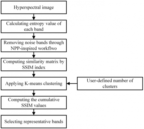
The proposed method comprises two steps of noisy bands removal and informative bands selection, and Figure 1 shows the workflow of the proposed FS algorithm.
In the first step, the entropy value of each hyperspectral band was calculated based on Eq. (1):
entropy $\left(b_{i}\right)=-\sum p\left(b_{i}\right) \log \mathrm{p}\left(b_{i}\right)$ (1)
where, bi and p(bi) are the ith band of the hyperspectral data and probability density function (PDF) of bi, respectively. When working with images, the ratio of the image histogram by the total number of pixels is considered as the PDF. The entropy value was recognized as a measure of randomness [21]. Accordingly, it was employed as a criterion to investigate the randomness of an image [22]. Therefore, this measure can be utilized to separate noisy bands of the hyperspectral data since their degree of randomness is different in comparison with pure bands. To this end, the entropy values of hyperspectral bands were applied to a Normal Probability Plot (NPP) inspired workflow to determine the noisy bands. The NPP is a statistical approach that enables the identification of outliers (i.e., noisy bands) from pure data [23]. Since the hyperspectral observations follow normality, it was presumed that their entropy values should follow normality [24]. The cumulative probabilities and their corresponding normal scores were computed to produce an NPP. Finally, instead of using a theoretical normal distribution, a Normal Probability Distribution (NPD) was fitted to the entropy values and their corresponding normal scores. This modification facilitated the determination of noisy bands. In fact, the fitted NPD would be a straight line, and the disparity from this line illustrates the departure of an entropy value from normality.
Figure 1. Flowchart of the proposed method for hyperspectral band selection and classification
After removing noisy bands, the SSIM index was applied to measure the similarity of the remaining hyperspectral bands, resulting in a similarity matrix. The similarity matrix is dÍd (d is the number of remaining bands) symmetric matrix containing the pair-wise SSIM values of hyperspectral bands. The SSIM approaches one when two bands are the same. In contrast, the SSIM approaches zero when two bands are dissimilar. SSIM index comprises three elements, as shown in Eq. (2):
$\operatorname{SSIM}\left(b_{i}, b_{j}\right)=\left[l\left(b_{i}, b_{j}\right)\right]^{\alpha} \cdot\left[c\left(b_{i}, b_{j}\right)\right]^{\beta} \cdot\left[s\left(b_{i}, b_{j}\right)\right]^{\gamma}$ (2)
where, l is the luminance (see Eq. (3)), c is the contrast (see Eq. (4)), and s is the structural similarity (see Eq. (5)). α, β and γ are the adjusting parameters that are used to define the relative importance of each element. In this study, all adjusting parameters were set the same to exploit the potential of three elements equally.
$l\left(b_{i}, b_{j}\right)=\frac{2 \mu_{b_{i}} \mu_{b_{j}}+C_{1}}{\mu_{b_{i}}^{2}+\mu_{b_{j}}^{2}+C_{1}}$ (3)
$c\left(b_{i}, b_{j}\right)=\frac{2 \sigma_{b_{i}} \sigma_{b_{j}}+C_{2}}{\sigma_{b_{i}}^{2}+\sigma_{b_{j}}^{2}+C_{2}}$ (4)
$s\left(b_{i}, b_{j}\right)=\frac{\sigma_{b_{i} b_{j}}+C_{3}}{\sigma_{b_{i}} \sigma_{b_{j}}+C_{3}}$ (5)
where, μb and σb are the mean intensity and standard deviation of intensity values of the corresponding bands, and $\sigma_{b_{i} b_{j}}$ is the covariance value between ith and jth bands. C1, C2 and C3 are the constant values that were used to avoid instability in the calculation of each component.
The advantage of the SSIM index compared to other similarity indices is that it was developed in a 2D approach. In other words, the SSIM index measures the similarity of two bands locally and preserve the 2D image structure [19], whereas other similarity measures (e.g., correlation and mutual information) treat images as signals and disrupt the image structure, which carries critical information. Furthermore, the SSIM index is relatively uncomplicated to implement while providing superior performance in comparison with other similarity indices [25, 26].
After calculating the similarity matrix, the k-means clustering algorithm was applied to cluster hyperspectral bands into N user-defined dissimilar sub-bands. Afterward, the cumulative SSIM value of each band within each sub-band was calculated. Finally, a band with the highest cumulative SSIM value was determined as the representative candidate from each sub-band. These steps resulted in a dataset with a lower dimension by preserving and removing discriminative and redundant bands, respectively. The computation of the cumulative SSIM value enabled the selection of a band that could be a suitable representative of the corresponding sub-band since it is highly similar to other bands.
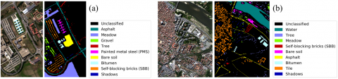
In this study, two well-known benchmark hyperspectral datasets were used to evaluate the performance of the proposed FS algorithm. Both datasets were captured by the Reflective Optics System Imaging Spectrometer (ROSIS) sensor in a 1.3 m spatial resolution. The first dataset was acquired in 102 bands over Pavia Centre, Italy, and the second dataset was captured in 103 bands over Pavia University, Italy. The former has a dimension of 1096Í715 pixels, and the latter has a size of 610Í340 pixels. Both datasets, along with their Ground Truth (GT) data, in nine classes, are shown in Figure 2. Two training sets comprising 20 (set 1) and 25 (set 2) samples per class were randomly collected from GT data for each dataset. Likewise, one independent test set containing 300 samples per class was selected for statistical assessment. The intention of employing a small number of training samples was to investigate the robustness of the proposed method when only a few samples are available.
Figure 2. Hyperspectral datasets of Pavia University (a) and Pavia Centre (b) with their corresponding GT data
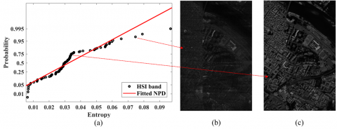
The proposed noisy band identification result, along with a sample noisy and pure band are shown in Figure 3. Figure 3(a) shows that most of the entropy values are closely at the sides of the fitted NPD, and only a few values are far from this line. Hyperspectral bands which their entropy values had a higher departure from the fitted NPD were identified as noisy bands and were removed for further steps. Furthermore, Figure 3(b) presents a sample noisy band in which the undesirable variation of the digital numbers made this band less informative. Its entropy value was more distant from the fitted NPD in comparison with other pure bands (e.g., Figure 3(c)). Moreover, a visual inspection was performed to ensure the correctness of the proposed noisy band identification approach. In this regard, all identified noisy bands were visually checked, and it was observed that the NPP-inspired workflow was correctly able to determine noisy bands.
After removing noisy bands, the proposed FS approach was applied to the remaining hyperspectral bands. Then, the selected bands were injected into the supervised classifier of SVM with a radial basis kernel function [27]. The obtained OA and KC were computed to evaluate the performance of different FS methods.
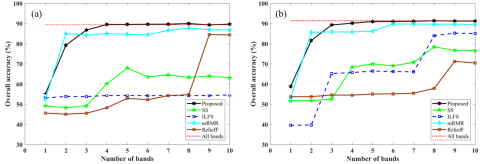
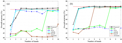
Figure 4 shows the achieved OAs of the Pavia Centre dataset when the selected features from five different FS algorithms are employed for classification. It is apparent that the proposed unsupervised FS method outperformed other supervised and unsupervised FS algorithms in nearly all steps. Furthermore, FS algorithms of SS, ReliefF, and ILFS were found to have weak performance, especially when a smaller number of training samples were employed. Moreover, the proposed method achieved higher classification accuracy in comparison with the case of exploiting all hyperspectral bands, indicating the capability of the proposed method to select discriminative bands. Likewise, the obtained OAs for Pavia University are presented in Figure 5. Figure 5 conveys that the proposed method not only achieved higher classification accuracy than other FS methods but also was able to attain better or similar results compared with the case of using all bands. The results illustrate that ReliefF (see Figure 5(a)) and ILFS (see Figure 5(b)) performed weakly in comparison with other methods. This performance may lie in the inherent characteristics of these supervised methods that require training samples, and they performed unstable when a small number of training samples were employed. Therefore, it can be stated that these methods are dependent on the number of training samples to be capable of selecting discriminative features.
The obtained results demonstrate the potential of the proposed algorithm for hyperspectral band selection and classification. Moreover, the proposed method proved to be more stable as the achieved OAs increased and became consistent in further steps, whereas other FS methods (e.g., SS, ILFS, and ReliefF) experienced several fluctuations, making them less stable. Additionally, Figures 4 and 5 illustrate a relatively similar behavior between the proposed and the mRMR FS methods. However, it should be noted that in addition to obtaining higher OA, the proposed method is an unsupervised FS algorithm, while the mRMR is a supervised approach. Therefore, the proposed approach is applicable when no reference samples are available. Furthermore, the proposed method effectively selected a few bands that achieved high OA and also reduced the computational complexity for training and applying the classifier, especially in the case of employing a small number of training samples [20].
Figure 3. Proposed NPP-inspired workflow for noisy band identification (a), sample noisy band (b), and sample pure band (c) for the Pavia Centre dataset
Figure 4. Obtained overall accuracies of different FS algorithms and all hyperspectral bands of the Pavia Centre dataset using training set 1 (a) and set 2 (b)
Figure 5. Obtained overall accuracies of different FS algorithms and all hyperspectral bands of the Pavia University dataset using training set 1 (a) and set 2 (b)
Table 1. Best-obtained overall accuracies and kappa coefficients of different FS algorithms and all hyperspectral bands
|
Dataset |
Training set |
Quantity measure |
All |
ILFS |
SS |
mRMR |
ReliefF |
SM |
Proposed |
|
Pavia Centre |
Set 1 |
OA (%) |
89.33 |
54.59 |
67.96 |
87.81 |
84.55 |
86.11 |
90.00 |
|
KC |
0.880 |
0.489 |
0.639 |
0.869 |
0.826 |
0.843 |
0.887 |
||
|
Set 2 |
OA (%) |
91.40 |
87.29 |
78.44 |
89.77 |
53.62 |
89.74 |
91.37 |
|
|
KC |
0.903 |
0.857 |
0.671 |
0.885 |
0.478 |
0.884 |
0.902 |
||
|
Pavia University |
Set 1 |
OA (%) |
70.96 |
70.55 |
70.81 |
70.88 |
54.85 |
69.51 |
72.85 |
|
KC |
0.673 |
0.668 |
0.671 |
0.672 |
0.491 |
0.657 |
0.694 |
||
|
Set 2 |
OA (%) |
74.03 |
72.92 |
73.07 |
73.81 |
54.14 |
73.25 |
74.37 |
|
|
KC |
0.707 |
0.695 |
0.697 |
0.705 |
0.482 |
0.69 |
0.711 |
Figure 6. Box plots of the obtained overall accuracies from 20 repeating times of each step for Pavia Centre (a) and Pavia University (b)
Table 2. Standard deviation values of obtained overall accuracies from 20 repeating times
|
Number of bands |
1 |
2 |
3 |
4 |
5 |
6 |
7 |
8 |
9 |
10 |
|
Pavia Centre |
||||||||||
|
SD (%) |
0.00 |
0.15 |
0.03 |
0.17 |
0.21 |
0.29 |
0.30 |
0.28 |
0.19 |
0.18 |
|
Pavia University |
||||||||||
|
SD (%) |
0.00 |
0.00 |
0.03 |
0.09 |
0.24 |
0.40 |
0.28 |
0.57 |
0.52 |
0.53 |
The best-obtained OAs of the mentioned Fs methods for Pavia Centre and Pavia University are provided in Table 1. The proposed FS method improved the classification results between 2.5% (1.7%) and 64.8% (70.4%) employing training set 1 (2) for the Pavia Centre dataset. Likewise, the classification results of Pavia University were refined between 2.6% (0.07%) and 32.8% (37.3%) using training set 1 (2) when the proposed FS approach was applied. Moreover, the proposed FS approach was capable of achieving higher OA and KC in comparison to the SM FS algorithm. It should be noted that the results of the SM algorithm are only provided in Table 1, as this method only returns a set of sub-band. Additionally, Table 1 indicates that the proposed FS algorithm obtained better or similar OA and KC in comparison with using all hyperspectral bands, while approximately 10% of bands were employed for classification.
Since the proposed method employed a clustering algorithm, a stability analysis was essential to assess the consistency of the selected features. This is rooted in the inherent characteristics of the k-means algorithm in which the final result is dependent on initial seeds. In other words, as the initial seeds change, the final clustering result change. In this regard, each step was repeated 20 times, and the obtained OAs were used to generate box plots. Figure 6 shows the stability analysis of the proposed FS algorithm based on the achieved OAs. The interquartile ranges (the difference between the first and the third quartiles) of almost all steps were lower than 1%, illustrating a low variability in obtained OA values [28]. The compactness of the interquartile ranges suggests the consistency of the proposed FS method. Furthermore, the whisker ranges also indicate the same variation, as they were lower than 2% in all steps. Moreover, the Standard Deviation (SD) of obtained OAs were computed (see Table 2). From Table 2, it is inferred that the proposed FS algorithm acquired reasonable stability in all steps since the highest SD values were 0.30% and 0.57% for Pavia Centre and Pavia University, respectively.
This study presents an unsupervised FS method for hyperspectral band selection. Entropy and the SSIM index were employed to remove noisy bands and select informative bands, respectively. The manual assessment revealed that the noisy band removal procedure successfully determined the noisy bands. Moreover, the proposed approach efficiently selects discriminative bands by removing redundant and preserving suitable bands. The selected bands were applied to an SVM classifier, and the results were evaluated based on OA and KC criteria. The results indicated that the proposed FS algorithm was able to improve the classification accuracy of two benchmark hyperspectral images in comparison with other well-known and state-of-the-art FS methods. Furthermore, the effectiveness of the proposed method was proved as it was capable of selecting a few bands while resulting in equal or higher classification accuracy in comparison with exploiting all hyperspectral bands. Finally, a stability analysis was performed to investigate the consistency of the proposed FS method, which confirmed a satisfactory stable manner. The proposed method can be efficiently applied to other hyperspectral images to select a few discriminative bands, which can result in acceptable OA, especially when a small number of training samples are available.
[1] Ghorbanian, A., Kakooei, M., Amani, M., Mahdavi, S., Mohammadzadeh, A., Hasanlou, M. (2020). Improved land cover map of Iran using sentinel imagery within google earth engine and a novel automatic workflow for land cover classification using migrated training samples. ISPRS Journal of Photogrammetry and Remote Sensing, 167: 276-288. https://doi.org/10.1016/j.isprsjprs.2020.07.013
[2] Amani, M., Kakooei, M., Moghimi, A., Ghorbanian, A., Ranjgar, B., Mahdavi, S., Davidson, A., Fisette, T., Rollin, P., Brisco, B. and Mohammadzadeh, A. (2020). Application of google earth engine cloud computing platform, sentinel imagery, and neural networks for crop mapping in Canada. Remote Sensing, 12(21): 3561. https://doi.org/10.3390/rs12213561
[3] Saleem, M.S., Ahmad, S.R., Javed, M.A. (2020). Impact assessment of urban development patterns on land surface temperature by using remote sensing techniques: a case study of Lahore, Faisalabad and Multan district. Environmental Science and Pollution Research, 27(32): 39865-39878. https://doi.org/10.1007/s11356-020-10050-5
[4] Ghorbanian, A., Sahebi, M.R., Mohammadzadeh, A. (2019). Optimization approach to retrieve soil surface parameters from single-acquisition single-configuration SAR data. Comptes Rendus Geoscience, 351(4): 332-339. https://doi.org/10.1016/j.crte.2018.11.005
[5] Janalipour, M., Mohammadzadeh, A. (2018). Evaluation of effectiveness of three fuzzy systems and three texture extraction methods for building damage detection from post-event LiDAR data. International Journal of Digital Earth, 11(12): 1241-1268. https://doi.org/10.1080/17538947.2017.1387818
[6] Beirami, B.A., Mokhtarzade, M. (2019). Spatial-spectral random patches network for classification of hyperspectral images. Traitement du Signal, 36(5): 399-406. https://doi.org/10.18280/ts.360504
[7] Gao, J., Meng, B., Liang, T., Feng, Q., Ge, J., Yin, J., Wu, C., Cui, X., Hou, M., Liu, J., Xie, H. (2019). Modeling alpine grassland forage phosphorus based on hyperspectral remote sensing and a multi-factor machine learning algorithm in the east of Tibetan Plateau, China. ISPRS Journal of Photogrammetry and Remote Sensing, 147: 104-117. https://doi.org/10.1016/j.isprsjprs.2018.11.015
[8] Kishore, D., Rao, C.S. (2020). A multi-class SVM based content based image retrieval system using hybrid optimization techniques. Traitement du Signal, 37(2): 217-226. https://doi.org/10.18280/ts.370207
[9] Paul, A., Chaki, N. (2019). Dimensionality reduction using band correlation and variance measure from discrete wavelet transformed hyperspectral imagery. Annals of Data Science, 1-14. https://doi.org/10.1007/s40745-019-00210-x
[10] Paul, A., Chaki, N. (2020). Dimensionality reduction of hyperspectral image using signal entropy and spatial information in genetic algorithm with discrete wavelet transformation. Evolutionary Intelligence. https://doi.org/10.1007/s12065-020-00460-2
[11] Ghorbanian, A., Mohammadzadeh, A. (2018). An unsupervised feature extraction method based on band correlation clustering for hyperspectral image classification using limited training samples. Remote Sensing Letters, 9: 982-991. https://doi.org/10.1080/2150704X.2018.1500723
[12] Jia, X., Kuo, B.C., Crawford, M.M. (2013). Feature mining for hyperspectral image classification. Proceedings of the IEEE, 101(3): 676-697. https://doi.org/10.1109/JPROC.2012.2229082
[13] Li, S., Zheng, Z., Wang, Y., Chang, C., Yu, Y. (2016). A new hyperspectral band selection and classification framework based on combining multiple classifiers. Pattern Recognition Letters, 83: 152-159. https://doi.org/10.1016/j.patrec.2016.05.013
[14] Rashwan, S., Dobigeon, N. (2017). A split-and-merge approach for hyperspectral band selection. IEEE Geoscience and Remote Sensing Letters, 14(8): 1378-1382. https://doi.org/10.1109/LGRS.2017.2713462
[15] Peng, H., Long, F., Ding, C. (2005). Feature selection based on mutual information criteria of max-dependency, max-relevance, and min-redundancy. IEEE Transactions on Pattern Analysis and Machine Intelligence, 27(8): 1226-1238. https://doi.org/10.1109/TPAMI.2005.159
[16] Liu, M., Zhang, D. (2014). Sparsity score: A novel graph-preserving feature selection method. International Journal of Pattern Recognition and Artificial Intelligence, 28(4): 1450009. https://doi.org/10.1142/S0218001414500098
[17] Roffo, G., Melzi, S., Castellani, U., Vinciarelli, A. (2017). Infinite latent feature selection: A probabilistic latent graph-based ranking approach. In Proceedings of the IEEE International Conference on Computer Vision, pp. 1398-1406. https://doi.org/10.1109/ICCV.2017.156
[18] Robnik-Šikonja, M., Kononenko, I. (2003). Theoretical and empirical analysis of ReliefF and RReliefF. Machine Learning, 53(1-2): 23-69. https://doi.org/10.1023/A:1025667309714
[19] Wang, Z., Bovik, A.C., Sheikh, H.R., Simoncelli, E.P. (2004). Image quality assessment: from error visibility to structural similarity. IEEE Transactions on Image Processing, 13(4): 600-612. https://doi.org/10.1109/TIP.2003.819861
[20] Wang, Q., Jianzhe L., Yuan Y. (2016). Salient band selection for hyperspectral image classification via manifold ranking. IEEE Transactions on Neural Networks and Learning Systems, 27(6): 1279-1289. https://doi.org/10.1109/TNNLS.2015.2477537
[21] Kvålseth, T.O. (2016). On the measurement of randomness (uncertainty): A more informative entropy. Entropy, 18(5): 159. https://doi.org/10.3390/e18050159
[22] Wu, Y., Zhou, Y., Saveriades, G., Agaian, S., Noonan, J.P., Natarajan, P. (2013). Local Shannon entropy measure with statistical tests for image randomness. Information Sciences, 222: 323-342. https://doi.org/10.1016/j.ins.2012.07.049
[23] Parsons, S., Flack, H.D., Wagner, T. (2013). Use of intensity quotients and differences in absolute structure refinement. Acta Crystallographica Section B: Structural Science, Crystal Engineering and Materials, 69(3): 249-259. https://doi.org/10.1107/S2052519213010014
[24] Manolakis, D.G., Marden, D., Kerekes, J.P., Shaw, G.A. (2001). Statistics of hyperspectral imaging data. In Algorithms for Multispectral, Hyperspectral, and Ultraspectral Imagery VII, 4381: 308-316. https://doi.org/10.1117/12.437021
[25] Wang, Z., Bovik, A.C., Simoncelli, E.P. (2005). Structural approaches to image quality assessment. Handbook of Image and Video Processing, 7: 18. https://doi.org/10.1016/B978-012119792-6/50119-4
[26] Bull, D.R. (2014). Communicating Pictures: A Course in Image and Video Coding. Academic Press.
[27] Cortes, C., Vapnik, V. (1995). Support-vector networks. Machine Learning, 20(3): 273-297. https://doi.org/10.1007/BF00994018
[28] Ferreira, J.E.V., Pinheiro, M.T.S., dos Santos, W.R.S., da Silva Maia, R. (2016). Graphical representation of chemical periodicity of main elements through boxplot. Educación Química, 27(3): 209-216. https://doi.org/10.1016/j.eq.2016.04.007