Nan Xiao* | Xinyue Zhang
© 2020 IIETA. This article is published by IIETA and is licensed under the CC BY 4.0 license (http://creativecommons.org/licenses/by/4.0/).
OPEN ACCESS
Flexible start-up is the future trend of production automation. To realize intelligent and flexible operations, industrial robot must position the target rapidly and accurately. Otherwise, it is impossible for the robot to operate automatically in complex environment. This paper designs a novel target positioning method that enables industrial robot to position its target with high precision and fast speed. Firstly, the target images were preprocessed through enhancement, histogram equalization, and filtering. Next, the target motion areas (TMAs) captured by the system of multiple visual sensors (MVSs) were subject to information fusion, and the feature points of fused image were matched and optimized. After that, the fused image was recognized and described by speeded up robust features (SURF)- fast retina key- point (FREAK) algorithm. Finally, a two-dimensional (2D) data model was established based on the centroid coordinates of the fused image. Experimental results prove that our method can effectively and accurately position target in complex environment, while simplifying size measurement and speeding up computation. The research results provide a reference for image collection and information fusion by MVSs system in other fields.
industrial robot, multiple visual sensors (MVSs), target positioning, feature point matching
As artificial intelligence (AI) permeates into industrial scenarios, machine vision has exhibited a great application potential in the field of industrial robot [1-6]. To realize intelligent and flexible operations, industrial robot must process the image of the target workpiece, position the target with a high precision, and move to the target rapidly and accurately. However, it is impossible to meet the precision required for target positioning with a single visual sensor (SVS) [7-18].
Currently, most industrial robots rely on a system of multiple visual sensors (MVSs) to collect images, fuse related information, and position the target. Many experts and scholars have explored the target positioning by MVSs system [19-22]. For example, Liu et al. [23] segmented the target image by principal component analysis (PCA) and wavelet transform, and created a rope model for industrial robot to locate and grasp the target. Li et al. [24] combined pyramid transform and wavelet transform, and constructed triangular grids to search for multiple grasp positions. Compared with a single grasping position, the multiple grasp positions help to keep the grasping strategy consistent. Through Contourlet transform, Rana et al. [25] set up a workpiece model library for industrial robot, and improved the target positioning by matching salient feature points between two or more workpiece model images.
This paper designs a novel MVSs-based target positioning method for industrial robot, aiming to optimize the information fusion of the MVSs system, and make the positioning by industrial robot more accurate and rapid. Firstly, the target images were preprocessed through enhancement, histogram equalization, and filtering. On this basis, the target motion area (TMA) of each SVS was confirmed, and the information of MVSs was fused. Then, the feature points of the fused image were matched and optimized. Next, the fused image was recognized and described by speeded up robust features (SURF)- fast retina key- point (FREAK) algorithm, which is an improved SURF algorithm. Finally, a two-dimensional (2D) data model was established based on the centroid coordinates of the fused image, completing the accurate positioning of target in complex environment. Our method was proved valid and accurate through experiments.
In the working environment of industrial cameras, illumination difference and overlapped objects are common defects arising from camera quality issue or lens imbalance. Sometimes, the imaging quality and target positioning are dampened by the performance of visual sensors. All these defects are unfavorable for subsequent operations, namely, feature point extraction from target images and target positioning for industrial robot. Therefore, the target images captured by industrial cameras should be enhanced and filtered.
Many metal components are highly reflective. In their images, the surface and edge features are easily affected by uneven brightness. Hence, the target images should firstly subject to brightness correction. Here, the target images are converted from the red-green-blue (RGB) space to the illuminance-chrominance (YCbCr) space:
$\left[ \begin{matrix} Y \\ Cb \\ Cr \\\end{matrix} \right]=\left[ \begin{matrix} 16 \\ 128 \\ 128 \\\end{matrix} \right]+\frac{1}{256}\left[ \begin{matrix} 65.738 & 125.097 & 25.068 \\ -37.148 & -74.291 & 112.439 \\ 112.439 & -94.368 & -18.071 \\\end{matrix} \right]\left[ \begin{matrix} R \\ G \\ {{B}'} \\\end{matrix} \right]$ (1)
$\left[ \begin{matrix} R \\ G \\ B \\\end{matrix} \right]=\frac{1}{256}\left[ \begin{matrix} 298.164 & 0 & 408.596 \\ 298.164 & -100.392 & -208.813 \\ 298.164 & 516.017 & 0 \\\end{matrix} \right]\left[ \begin{matrix} Y-16 \\ Cb-128 \\ Cr-128 \\\end{matrix} \right]$ (2)
Then, the boundary features of the target were enhanced by adjusting the illuminance (Y) value.
Next, the grayscale of each target image was enhanced by histogram equalization. The probability density functions before and after the equalization, Pori(x) and Penh(y), satisfy the following relationship:
$\int_{{{x}_{\min }}}^{{{x}_{\max }}}{{{P}_{ori}}\left( x \right)}dx=\int_{{{y}_{\min }}}^{{{y}_{\max }}}{{{P}_{enh}}\left( y \right)}dy$ (3)
In essence, histogram equalization requires Pori(x) outputs to obey balanced distribution:
${{P}_{ori}}\left( x \right)=1/\left( {{x}_{\max }}-{{x}_{\min }} \right),{{x}_{\min }}\le x\le {{x}_{\max }}$ (4)
The above two formulas can be combined into the formula of histogram equalization:
$B=\left( {{x}_{\max }}-{{x}_{\min }} \right){{P}_{enh}}\left( y \right)+{{x}_{\min }}$ (5)
After equalization, the target images were reversely converted from the YCbCr space to the RGB space:
$\left[ \begin{matrix} R \\ G \\ B \\\end{matrix} \right]=\frac{1}{256}\left[ \begin{matrix} 298.164 & 0 & 408.596 \\ 298.164 & -100.392 & -208.813 \\ 298.164 & 516.017 & 0 \\\end{matrix} \right]\left[ \begin{matrix} Y-16 \\ Cb-128 \\ Cr-128 \\\end{matrix} \right]$ (6)
The brightness polynomial for each new target image was established, on the premise that the saliency and brightness of the image can be adjusted arbitrarily.
In addition, noises are inevitably included in the images through acquisition, generation, transmission and storage. Here, the noises are filtered by a 5×5 Gaussian filter:
$g\left( x,y \right)=\frac{1}{2\pi {{\sigma }^{2}}}{{e}^{-\frac{{{x}^{2}}+{{y}^{2}}}{2{{\sigma }^{2}}}}}$ (7)
where, σ is the variance of the Gaussian function, reflecting filtering smoothness. During Gaussian filtering, the template was processed into integers, which speeds up computation without sacrificing noise suppression and feature preservation.
To highlight boundary and salient features and prevent local grayscale mutations, the Laplacian edge sharpening algorithm was adopted to sharpen the fuzzy edges on the filtered images:
$\begin{align} & {I}'\left( x,y \right)=I\left( x,y \right)-{{\nabla }^{2}}\left( x,y \right) \\ & \begin{matrix} {} & {} & =5I\left( x,y \right)-\left[ I\left( x+1,y \right)+I\left( x-1,y \right)+I\left( x,y+1 \right)+I\left( x,y-1 \right) \right] \\\end{matrix} \\\end{align}$ (8)
${{\nabla }^{\text{2}}}\left( x,y \right)=\left[ I\left( x+1,y \right)+I\left( x-1,y \right)+I\left( x,y+1 \right)+I\left( x,y-1 \right) \right]-4I\left( x,y \right)$ (9)
The MVSs-based target detection and tracking follows a similar process as the SVS-based approach. As shown in Figure 1, this paper confirms the TMA of the image outputted by each visual sensor, fuses the images captured by the MVSs, extract the salient features from the fused image, and optimizes the target position through feature point matching, thereby recognizing the target and its position information.
Figure 1. The workflow of target detection and tracking
3.1 Confirming TMA of each SVS
Dynamic target detection based on visual sensors is the basis of industrial robot target positioning. The performance of the sensor network, coupled with the accuracy of target detection, affects the effects of subsequent operations like target positioning and tracking. To realize dynamic target detection, the detection method must support real-time response and feature strong robustness.
For simple and rapid detection and tracking of dynamic target, the target image I' (x, y) captured by each visual sensor at time t+1 was subtracted from that I(x, y) captured by that sensor at the current time t, creating the binary difference diagram of that sensor at time t+1:
$D(x, y)=\left\{\begin{array}{ll}1 & \left|I^{\prime}(x, y)-I(x, y)\right| \geq T_{t} \\ 0 & \left|I^{\prime}(x, y)-I(x, y)\right|<T_{t}\end{array}\right.$ (10)
where, Tt is the threshold of pixel I(x, y) at the current moment. The TMA of each SVS can be determined by the difference operation above and threshold comparison. To mitigate the noise induced by uneven illumination and lens imbalance, the threshold was determined adaptively by:
${{T}_{t+1}}=u{{T}_{t}}+\left( 1-u \right)\left| {I}'\left( x,y \right)-I\left( x,y \right) \right|$ (11)
where, u is the update speed coefficient of the adaptive threshold, which is negatively correlated with the update speed at time Tt.
3.2 MVSs information fusion
Based on the detection result and confidence of each SVS, the information from MVSs was fused by fuzzy integral operation. The binary difference result of the i-th sensor in the time interval [t, t+n] can be expressed as:
${{D}_{i}}={{\left( {{d}_{it}},{{d}_{i(t+1)}},\cdots ,{{d}_{i(t+n)}} \right)}^{T}}$ (12)
where, di(t+j) is the output of the binary difference model at time j, reflecting the degree of correlation between the output of the i-th sensor and the predicted TMA at time j.
Let hi be the confidence of the i-th sensor. Then, the mapping function for the set Ci of m visual sensors to predict the TMA at time j can be defined as:
${{K}_{j}}\left( {{C}_{i}} \right)={{h}_{i}}{{d}_{i}}$ (13)
Let μi be the reliability of the binary difference model of the i-th sensor, and μ(●) is the fuzzy measure relative to μδ in set Ci. Then, the fuzzy integral of the fuzzy measure μ(●) in the above mapping function can be expressed as:
${{\lambda }_{j}}={{K}_{j}}\left( {{C}_{i}} \right)\circ \mu \left( \bullet \right)=\underset{{{C}_{i}}\subset C}{\mathop{\max }}\,\left[ \min \left( \underset{a\in {{N}_{i}}}{\mathop{\min }}\,{{K}_{j}}\left( a \right),\mu \left( {{C}_{i}} \right) \right) \right]$ (14)
μi needs to satisfy the following constraints:
$\mu \left( {{C}_{1}} \right)={{\mu }_{1}}$
$\mu ({{C}_{i}})={{\mu }_{i}}+\mu \left( {{C}_{i-1}} \right)+\delta {{\mu }_{i}}\mu \left( {{C}_{i-1}} \right)$ (15)
$1+\delta =\underset{i=1}{\overset{m}{\mathop{\prod }}}\,(1+\delta {{\mu }_{i}})$
The fuzzy integral λj is a measure of the probability that the MVSs system judges an area as the TMA at time j in the time interval of [t, t+n].
Through the fusion of MVSs information, the optimal TMA and confidence can be derived from the TMAs identified by different visual sensors and the confidences of the binary difference models for different sensors.
Tables 1 and 2 below provide the measured values, binary differences, and confidences of the ten sensors used in our experiments.
Table 1. Parameters of MVSs after information fusion
|
Sensor number |
Measured value/cm |
Binary difference/cm |
Sensor number |
Measured value/cm |
Binary difference/cm |
|
1 |
1.030 |
0.05 |
6 |
1.433 |
0.44 |
|
2 |
0.946 |
0.08 |
7 |
1.783 |
0.15 |
|
3 |
0.976 |
0.23 |
8 |
1.567 |
0.07 |
|
4 |
0.925 |
0.25 |
9 |
1.335 |
0.21 |
|
5 |
1.845 |
0.06 |
10 |
1.673 |
0.08 |
Table 2. Confidences of MVSs after information fusion
|
Sensor number |
Confidence |
Sensor number |
Confidence |
|
1 |
0.137 |
6 |
0.275 |
|
2 |
0.156 |
7 |
0.197 |
|
3 |
0.165 |
8 |
0.096 |
|
4 |
0.159 |
9 |
0.172 |
|
5 |
0.126 |
10 |
0.115 |
3.3 MVSs-based feature point matching and optimization
In the MVSs system, the target images are collected by different sensors. The source difference may lead to huge differences between images in illumination, angular change and scale. Therefore, the algorithm that matches the feature points with the template must have high robustness and strong anti-interference ability. Considering the sheer number of images outputted by the MVSs system, the algorithm should be able to match feature points rapidly. For these reasons, this paper chooses the SURF-FREAK algorithm to identify and describe the target images captured by the MVSs on industrial robot. The SURF algorithm mimics the 2D discrete wavelet transform response and makes effective use of the integral graph. Each original target image was integrated to obtain the grayscale intensity of pixels in any rectangular area. The sum of grayscales in the rectangular area with the upper left corner and pixel I(x, y) as two opposing corners can be expressed as:
${{I}_{\sum x,y}}=\sum\limits_{i=0}^{i\le x}{\sum\limits_{j=0}^{j\le y}{I\left( x,y \right)}}$ (16)
$Det\left( {{H}_{app}} \right)={{O}_{xx}}{{O}_{yy}}={{\left( 0.9{{O}_{xy}} \right)}^{2}}$ (17)
where, Oxx, Oxy and Oyy are the convolution results of the template and the image; Det(Happ) is the filter response of the rectangular area around P(a, b). The extreme points being detection can be used to compute the rectangular trajectory.
By changing the size of the rectangular area of the template, the filter responses of the Hessian matrix were computed based on the template and the integral image of different sizes. Then, the salient features of the target image on different scales were calculated from the response images.
On this basis, the Harr wavelet response operation was performed on the circular neighborhood of each feature point, whose radius is six times the scale of that point. The response values in x and y directions at any neighboring point were Gaussian weighted, such that the wavelet responses at neighboring points are positively correlated with their distances to the feature point.
After that, the responses of all neighboring points were summed to form a 60-degree fan-shaped area. The direction with the largest sum of responses in the circular neighborhood was taken as the main direction of that feature point. Hence, the feature point description operator of the SURF algorithm can be obtained as:
${{\upsilon }_{sub}}=\left( \sum{da,\sum{db,\sum{\left| da \right|,\sum{\left| db \right|}}}} \right)$ (18)
The 20s×20s rectangular model, which was established in the main direction of the feature point, was divided into 16 equal 5s×5s rectangular blocks. The Harr wavelet responses of every blocks were computed, and added up into a four-dimensional (4D) vector υsub.
To meet the real-time requirements of actual situations, the efficiency of the SURF feature point description operator should be further improved. In this paper, the feature points of each target image extracted by the SURF algorithm are described by the FREAK local description operator based on binary bit string:
$F=\sum\limits_{0\le a\le N}{{{2}^{a}}T({{P}_{a}})}$ (19)
where, T(Pa) is a smooth intensity function; Pa is a pair of sample points. Let f(Pa) be the grayscale of a sampling point after Gaussian blurring. The following constraint can be established:
$T({{P}_{a}})=\left\{ \begin{matrix} 1,\text{ }f(P_{a}^{\tau 1})\text{}f(P_{a}^{\tau 2})\text{ } \\ 0,f(P_{a}^{\tau 1})\le f(P_{a}^{\tau 2})\text{ } \\\end{matrix} \right.$ (20)
In the neighborhood of a feature point, there might be dozens of sampling point. Thus, the total number of sampling point pairs could reach tens of hundreds. The sampling point pairs must be filtered to retain useful information.
Firstly, a matrix of P feature points of the target image was constructed W=[W1, W2, …, WP]T. In the matrix, the k-th row contains the comparison results of l sampling point pairs in the neighborhood of the k-th feature point. Note that l is also the number of columns in that matrix.
Next, the mean value of each column in the matrix was computed. To obtain unique features, the columns with small variances were removed, leaving those with large variances. Finally, the Hausdorff distance was taken as the similarity measure to complete the matching of feature points.
The key to target positioning by industrial robot is to establish a centroid coordinate system for the target. During feature point matching, errors might occur due to translation, rotation or scaling.
To control the errors, this paper sets up a 2D scale data model based on the centroid coordinates of the target image. The model simplifies the size measurement and calculation of the target workpiece, making it possible to accurately position the target in complex environment.
The centroid coordinates of a graph formed by T reference points can be expressed as:
$CEN\left( x,y \right)=\left( \frac{{{x}_{1}}+{{x}_{2}}+\cdots +{{x}_{T}}}{T},\frac{{{y}_{1}}+{{y}_{2}}+\cdots +{{y}_{T}}}{T} \right)$ (21)
It can be seen that the centroid, lying at the geometric center of the image, is the mean coordinates of all reference points.
In actual situations, the image acquisition and boundary processing of visual sensors are affected by various factors, such as illumination, jitter, occlusion, and noise. These influencing factors bring about computing errors, and slow down the measurement and positioning.
Since an intersection can be defined by three circles, three reference points A(x1, y1), B(x2, y2) and C(x3, y3) were selected to determine the boundary features between template and target image. The distances of the three points to the centroid coordinates Cen(x, y) are r1, r2 and r3, respectively. Then, we have:
$\left[ \begin{matrix} x \\ y \\\end{matrix} \right]={{\left[ \begin{matrix} 2({{x}_{1}}-{{x}_{3}}) & 2({{y}_{1}}-{{y}_{3}}) \\ 2({{x}_{2}}-{{x}_{3}}) & 2({{y}_{1}}-{{y}_{3}}) \\\end{matrix} \right]}^{-1}}\left[ \begin{matrix} x_{1}^{2}-x_{3}^{2}+y_{1}^{2}-y_{3}^{2}-r_{1}^{2}+r_{3}^{2} \\ x_{2}^{2}-x_{3}^{2}+y_{2}^{2}-y_{3}^{2}-r_{2}^{2}+r_{3}^{2} \\\end{matrix} \right]$ (22)
By the above formula, the intersection points (xAB1, yAB1) and (xAB2, yAB2) between the circle with A(x1, y1) as the center and r1 as the radius and the circle with B(x2, y2) as the center and r2 as the radius were determined, and the closer one between the two intersection points to C(x3, y3) was selected and denoted as (xAB, yAB).
Similarly, the intersection points (xAC1, yAC1) and (xAC2, yAC2) between the circle with A(x1, y1) as the center and r1 as the radius and the circle with C(x3, y3) as the center and r3 as the radius were determined, and the closer one between the two intersection points to B(x2, y2) was selected and denoted as (xAC, yAC).
Furthermore, the intersection points (xBC1, yBC1) and (xBC2, yBC2) between the circle with B(x2, y2) as the center and r2 as the radius and the circle with C(x3, y3) as the center and r3 as the radius were determined, and the closer one between the two intersection points to A(x1, y1) was selected and denoted as (xBC, yBC).
Then, the geometric center of the intersection of the three circles was taken as the centroid, whose coordinates can be expressed as:
$CEN\left( {x}',{y}' \right)=\left( \frac{{{x}_{AB}}+{{x}_{AC}}+{{x}_{BC}}}{3},\frac{{{y}_{AB}}+{{y}_{AC}}+{{y}_{BC}}}{3} \right)$ (23)
Because the targets of industrial robots are often irregular in shape, the minimum bounding box method was adopted to measure the size of the target workpiece after determining the centroid position.
Firstly, a simple bounding box, parallel to the x or y axis, was constructed for the target workpiece. Next, the CEN(x¢¢, y¢¢) coordinates were calculated after a point (x0, y0) on the image plane has rotated by an angle θ about the fixed point CEN(x¢, y¢):
$\begin{matrix} {x}''=({x}'-{{x}_{0}})\cos \theta -({y}'-{{y}_{0}})\sin \theta +{{x}_{0}} \\ {y}''=({x}'-{{x}_{0}})\sin \theta +({y}'-{{y}_{0}})\cos \theta +{{y}_{0}} \\\end{matrix}$ (24)
The target workpiece was rotated by -90~90°. After rotation, the simple bounding box was obtained for the target workpiece. The area, vertex coordinates and the degree of rotation of this bounding box were recorded.
Then, all the simple bounding boxes obtained in the rotation process were compared, leaving only the smallest box. The vertex coordinates and rotation angle of the smallest box were recorded. After that, the smallest box was rotated by the same degree in the opposite direction. At the end of rotation, the smallest box became the minimum bounding box, and underwent length and width measurements.
Finally, the size of the target workpiece can be obtained by counting the pixel values on x and y axes:
$\begin{matrix} X=\sum\limits_{X=1}^{N}{I\left( x,y \right)} & Y=\sum\limits_{y=1}^{M}{I\left( x,y \right)} \\\end{matrix}$ (25)
The MVSs-based target positioning system for industrial robot consists of multiple parts (Figure 2). The image capturing systems collect, preprocess and store images on the target workpiece. These images are fused in information fusion module, and then subject to feature point matching against the workpiece template.
Figure 2. Structure of the MVSs-based target positioning system for industrial robot
(a) Before preprocessing; (b) After preprocessing
Figure 3. Histograms of a target image before and after preprocessing
Figure 3 compares the histograms of a target image before and after preprocessing. It can be seen that the preprocessing makes the probability density distribution more uniform, the grayscale greater, and the overall contrast more significant.
To verify the reliability of the proposed information fusion method, the MVSs system was applied to position four targets of different types. The measured values, binary differences, and confidences of the MVSs system are displayed in Tables 3 and 4.
Compared with the target detection by presetting the weight coefficients of MVSs, our method outputted objective and reasonable results, for it fully utilizes the image information collected by visual sensors.
Figure 4. Position errors of SVS-based and MVSs-based target detections
Figure 5. Angular errors of SVS-based and MVSs-based target detections
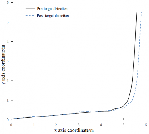
According to the target detection results, the robot moved from the start point to the target workpiece. The visual sensors captured data in real time throughout the motion. Figures 4 and 5 provide the position and angular errors of SVS-based and MVSs-based target detections, respectively. It can be seen that the MVSs-based target detection had the smaller position and angular errors. Figure 6 compares the robot trajectories before and after using our method. It is learned that the positioning accuracy of our method fully meets the requirement for industrial robot target positioning in industrial environment.
Figure 6. Robot trajectories before and after using our method
Table 3. Parameters of MVSs on 4 targets after information fusion
|
Sensor number |
Target 1 |
Target 2 |
Target 3 |
Target 4 |
||||
|
Measured value/cm |
Binary difference/cm |
Measured value/cm |
Binary difference/cm |
Measured value/cm |
Binary difference/cm |
Measured value/cm |
Binary difference/cm |
|
|
1 |
1.664 |
0.28 |
2.345 |
0.41 |
0.262 |
0.04 |
3.74 |
0.73 |
|
2 |
1.943 |
0.37 |
3.24 |
0.45 |
0.345 |
0.09 |
4.56 |
0.57 |
|
3 |
0.795 |
0.46 |
1.862 |
0.24 |
0.865 |
1.64 |
4.78 |
1.31 |
|
4 |
1.533 |
0.59 |
2.355 |
0.59 |
0.258 |
1.99 |
7.66 |
1.53 |
|
5 |
1.357 |
0.35 |
2.759 |
0.68 |
0.678 |
2.85 |
2.72 |
2.44 |
Table 4. Confidences of MVSs on four targets after information fusion
|
Sensor number |
Target 1 |
Target 2 |
Target 3 |
Target 4 |
|
1 |
0.284 |
0.525 |
0.554 |
0.033 |
|
2 |
0.431 |
0.638 |
0.047 |
0.636 |
|
3 |
0.570 |
0.412 |
0.622 |
0.740 |
|
4 |
0.746 |
0.439 |
0.702 |
0.129 |
|
5 |
0.457 |
0.211 |
0.531 |
0.120 |
This paper puts forward a novel MVSs-based target positioning method for industrial robot. The target images were preprocessed through enhancement, histogram equalization, and filtering, and then the TMA of each SVS was confirmed. Experimental results show that the preprocessing makes the probability density distribution more uniform, the grayscale greater, and the overall contrast more significant.
In addition, the information of the MVSs was fused, followed by matching and optimization of feature points in the fused image. After information fusion, the MVSs system was applied to detect four targets. According to the measured values, binary differences and confidences, the information fusion improves the objectiveness and reasonability of the positioning results.
Further, the fused image was recognized and described by SURF-FREAK algorithm, an improved SURF. Then, a 2D data model was established based on the centroid coordinates of the fused image. Experimental results prove that our method can accurately position target in complex environment, and that the positioning accuracy fully meets the requirement for industrial robot target positioning in industrial environment.
[1] Ge, Q., Shao, T., Yang, Q., Shen, X., Wen, C. (2016). Multisensor nonlinear fusion methods based on adaptive ensemble fifth-degree iterated cubature information filter for biomechatronics. Systems Man and Cybernetics, 46(7): 912-925. https://doi.org/10.1109/TSMC.2016.2523911
[2] Ghosh, D., Samanta, B., Chakravarty, D. (2017). Multi sensor data fusion for 6D pose estimation and 3D underground mine mapping using autonomous mobile robot. International Journal of Image and Data Fusion, 8(2): 173-187. https://doi.org/10.1080/19479832.2016.1226966
[3] Belmonte-Hernandez, A., Hernandez-Penaloza, G., Alvarez, F., Conti, G. (2017). Adaptive fingerprinting in multi-sensor fusion for accurate indoor tracking. IEEE Sensors Journal, 17(5): 4983-4998. https://doi.org/10.1109/JSEN.2017.2715978
[4] Shivanand, G., Reddy, K.V., Prasad, D. (2016). An innovative asynchronous, multi-rate, multi-sensor state vector fusion algorithm for air defence applications. IFAC-PapersOnLine, 49(1): 337-342. https://doi.org/10.1016/j.ifacol.2016.03.076
[5] Muniandi, G., Deenadayalan, E. (2019). Train distance and speed estimation using multi sensor data fusion. Iet Radar Sonar and Navigation, 13(4): 664-671. https://doi.org/10.1049/iet-rsn.2018.5359
[6] Sun, G.X., Bin, S., Jiang, M. (2019). Research on public opinion propagation model in social network based on blockchain. CMC-COMPUTERS MATERIALS & CONTINUA, 60(3): 1015-1027. http://dx.doi.org/10.32604/cmc.2019.05644
[7] Plangi, S., Hadachi, A., Lind, A., Bensrhair, A. (2018). Real-time vehicles tracking based on mobile multi-sensor fusion. IEEE Sensors Journal, 18(24): 10077-10084. https://doi.org/10.1109/JSEN.2018.2873050
[8] Kumar, S. (2016). Multi-sensordatafusion methods forindoor localization under collinear ambiguity. Pervas Mobile Comput, 9. https://doi.org/10.1016/j.pmcj.2015.09.001
[9] Al Hage, J., El Najjar, M.E., Pomorski, D. (2017). Multi-sensor fusion approach with fault detection and exclusion based on the Kullback–Leibler Divergence: Application on collaborative multi-robot system. Information Fusion, 37: 61-76. https://doi.org/10.1016/j.inffus.2017.01.005
[10] Zsedrovits, T., Bauer, P., Nemeth, M., Pencz, B.J.M., Zarandy, A., Vanek, B., Bokor, J. Performance analysis of camera rotation estimation algorithms in multi-sensor fusion for unmanned aircraft attitude estimation. 2015 Workshop on Research, Education and Development of Unmanned Aerial Systems (RED-UAS). https://doi.org/10.1109/RED-UAS.2015.7440991
[11] Nada, D., Bousbia-Salah, M., Bettayeb, M. (2018). Multi-sensor data fusion for wheelchair Position estimation with unscented Kalman filter. International Journal of Automation and Computing, 2.
[12] Al Hage, J., El Najjar, M.E., Pomorski, D. (2017). Multisensor fusion approach with fault detection and exclusion based on the Kullback–Leibler divergence: Application on collaborative multi-robot system. Information Fusion, 37 (2017): 61-76. https://doi.org/10.1016/jminffus.2017.01.005
[13] Surber, J., Teixeira, L.P., Chli, M. (2017). Robust visual-inertial localization with weak GPS priors for repetitive UAV flights. 2017 IEEE International Conference on Robotics and Automation (ICRA), May. https://doi.org/10.1109/ICRA.2017.7989745
[14] Hamdini, R., Diffellah, N., Namane, A. (2019). Robust local descriptor for color object recognition. Traitement du Signal, 36(6): 471-482. https://doi.org/10.18280/ts.360601
[15] Bin, S., Sun, G. (2020). Optimal energy resources allocation method of wireless sensor networks for intelligent railway systems. Sensors, 20(2): 482. https://doi.org/10.3390/s20020482
[16] Mukhopadhyay, B., Sarangi, S., Srirangarajan, S., Kar, S. Indoor localization using analog output of pyroelectric infrared sensors. IEEE Wireless Communications and Networking Conference, Barcelona, Spain. https://doi.org/10.1109/WCNC.2018.8377063
[17] Li, T.C., Prieto, J., Fan, H., Corchado, J.M. (2018). A robust multi-sensor PHD filter based on multi-sensor measurement clustering. IEEE Commun. Lett., 22(10): 2064-2067. https://doi.org/10.1109/LCOMM.2018.2863387
[18] Hosseinyalamdary, S. (2018). Deep Kalman filter: Simultaneous multi-sensor integration and modelling; A GNSS/IMU case study. Sensors, 18(5): 1316. https://doi.org/10.3390/s18051316
[19] Ruotsalainen, L., Kirkko-Jaakkola, M., Rantanen, J., Mäkelä, M. (2018). Error modelling for multi-sensor measurements in infrastructure-free indoor navigation. Sensors, 18(2): 29443918.
[20] Gabela, J., Kealy, A., Li, S.H., Hedley, M., Moran, W., Ni, W., Williams, S. (2019). The effect of linear approximation and Gaussian noise assumption in multi-sensor positioning through experimental evaluation. IEEE Sensors Journal, 19(22): 10719-10727. https://doi.org/10.1109/JSEN.2019.2930822
[21] Plangi, S., Hadachi, A., Lind, A., Bensrhair, A. (2018). Real-time vehicles tracking based on mobile multi-sensor fusion. IEEE Sensors Journal., 18(24): 10077-10084. https://doi.org/10.1109/JSEN.2018.2873050
[22] Li, J.H., Ito, A., Yaguchi, H., Maeda, Y. (2019). Simultaneous kinematic calibration, localization, and mapping (SKCLAM) for industrial robot manipulators. Advanced Robotics, 33: 1225-1234. https://doi.org/10.1080/01691864.2019.1689166
[23] Liu, H., Zhu, W.D., Dong, H.Y., Ke, Y.L. (2018). An improved kinematic model for serial robot calibration based on local POE formula using position measurement. The Industrial Robot, 45(5): 573-584. https://doi.org/10.1108/IR-07-2018-0141
[24] Li, Z.J., Huang, B., Ye, Z.F., Deng, M.D., Yang, C.G. (2018). Physical humanCrobot interaction of a robotic exoskeleton by admittance control. IEEE Transportation Industrial Electronics, 65(12): 9614-9624.
[25] Rana, R., Gaur, P., Agarwal, V., Parthasarathy, H. Tremor estimation and removal in robot-assisted surgery using lie groups and EKF. Robotica, 37(11): 1-18. https://doi.org/10.1017/S0263574719000341