Anu Bala* | Asha Rani | Sanjeev Kumar
© 2020 IIETA. This article is published by IIETA and is licensed under the CC BY 4.0 license (http://creativecommons.org/licenses/by/4.0/).
OPEN ACCESS
In this paper, a novel algorithm for face recognition is proposed in case of the images having illumination artifacts. First homomorphic filtering is done on the input face images to achieve partial illumination insensitivity. The fraction of the value of the image gradient to the original image intensity is evaluated to get an illumination independent normalized image. Here, gradient-domain is preferred since it explicitly accounts for the relationship between neighboring pixel points in the image. Then, Locality Sensitive Discriminant Analysis (LSDA) is applied to analyze the class relationship between data points. The proposed method performs very well, even if the number of training images is not sufficient. The experimental results on the extended Yale B database show that a significant improvement has been achieved in the recognition rate by making them illumination independent.
face recognition, image gradients, illumination normalization, reflectance model, LSDA
Face recognition is an important identity verification technique employed in several applications and areas such as police verification, access control, video surveillance, and many others. It is an assignment to make a true recognition of a face in a photograph or video against an already accessible dataset of faces. Face recognition starts with detection, proceeds with separating the human faces from other objects within the image and then identify those detected faces.
In the last decade, a noteworthy development has been made in the field of face recognition. However, the effectuation of most intelligent face recognition algorithms is very sensitive to the variation of lighting conditions. These algorithms may not perform very well under the illumination variation. Many approaches have been proposed to get rid of the illumination variation effects in recent years [1]. Now the idea of development of the illumination-invariant normalization approaches for face recognition has been described briefly. To the best of our knowledge, almost each technique for face identification under variable lighting conditions, followed the initiative work of Horn [2], and utilized the fact that the luminance of an image is usually smoother than the reflectance. It was assumed that the most illumination variation lies in the low frequency part of the spectrum. But later on, Xie et al. [3] explored that some of the important features for face recognition may rest in the low frequency part and so not advisable to discard that part. In general, illumination normalization techniques can be categorized into three groups.
The first group adopts image preprocessing techniques for normalizing face images under varying illumination conditions. Lee et al. [4], the orientated local histogram equalization (OLHE) has been proposed to compensate illumination, while preserving rich information on the edge orientations. Zhang et al. [5], the lighting invariant representation of the image was obtained by taking the ratio of the image gradients. Their approach was based upon the fact that the lighting component changes slowly as compared to the reflection component of an image. Impressed by the benefits of the gradient domain, Tzimiropoulos et al. [6] have also described a novel technique of subspace learning from image gradient orientations instead of image intensities for recognizing face images. Wang et al. [7], the illumination invariant face images were obtained by taking the tangent inverse of the ratio of the reflectance change to the original reflectance. The algorithm considered the neighborhood of the image pixels based upon Weber’s law for this purpose. Ding et al. [8], a robust approach to obtain “Multi-Directional Multi-Level Dual-Cross Patterns” (MDML-DCPs) from the face images, has been proposed. The authors used the Gaussian operator and its first derivative to make the input images illumination insensitive and then proposed a new face image descriptor based upon the textural structure of human faces.
The second group handles the illumination problem by considering the 3-D representation of face images. Kumar et al. [9], the authors have proposed a 3-D face recognition algorithm by making use of the orthogonal tensor locality sensitive discriminant analysis (OLSDA). Their algorithm was inspired by the Locality Sensitive Discriminant Analysis (LSDA) [10, 11]. LSDA maximizes the margin between data points that belong to different classes and minimize the distance between data points that belong to the same class. LSDA represents an image in the form of a one-dimensional vector that makes it challenging to reconstruct 3-D face data. So, Kumar et al. [9] have used tensor OLSDA to overcome this problem by evaluating the mutually orthogonal basis functions in the iterative aspect using tensor data representation.
The third group extracts the invariant illumination information from the given intensity images. Chen et al. [12] have employed the scale-invariant property of natural images to construct a Wiener filter which extracts illumination invariant features from the images. The non-sub-sampled contourlet transform (NSCT) has been investigated for face image recognition in da Cunha et al. [13]. Their algorithm was based upon the decomposition of the image into various frequency subbands. The obtained coefficients of these subbands were used for face recognition directly. Their algorithm was extended by taking NSCT in the logarithmic domain to extort the illumination invariant facial features in Xie et al. [14]. They concluded that the decomposition process could not correctly extract the facial features, as the reflectance model non linearly characterizes an image. Nabatchian et al. [15], a maximum filter was used to get invariant illumination images, and then mutual information (MI) and image entropy were incorporated as a weight factor for classifiers in face recognition. Their algorithm is also robust to the face recognition system in case of image occlusion. Cao et al. [16] extracted the invariant illumination information from the face images using wavelet coefficients in the logarithmic domain.
Zhang and Xie [17] concluded that the combination of image preprocessing and illumination invariant extraction is the best way to attain the satisfied face recognition. Hu et al. [18], the classification of image sets is proposed based upon the sparse approximate nearest points (SANP) for face recognition. The optimization of SANP in their algorithm accounts for the minimization of the distance and the maximization of the sparsity of the nearest points. Naseem et al. [19] formulated their approach for identification of face images in terms of linear regression, giving their results in case of varying facial expression and occlusion also. Anvaripour and Ebrahimnezhad [20], the local shape descriptors were used to obtain the boundary fragment extraction using Poisson equation properties. Afterward, the Gaussian mixture model (GMM) was employed to find the relation between boundary fragments and then finally detect the object. Biswas and Ghose [21], an algorithm based upon orientation histogram of Hough Transform Peaks has been proposed. Tan and Triggs [22], a method using local texture feature sets has been presented for face recognition in case of uncontrolled lighting conditions.
Deep learning is a foremost technique in machine learning. Deep Neural Networks (DNN) find many applications in the field of face recognition, image classification and speech recognition. A nice demonstration has been given in Balaban [23] about state of the art (SOTA) regarding deep learning and face recognition. Elmahmudi and Ugail [24] performed experiments by taking individual parts of the face like nose, eyes and cheeks and also by joining them. They used two classifiers viz. cosine similarity and linear support vector machines to find the recognition rates. Bah and Ming [25], Local Binary Pattern (LBP) has been employed for face recognition after preprocessing of the face images using histogram equalization, contrast adjustment and bilateral filter. Jin et al. [26], face recognition approach has been demonstrated using neural learning techniques, which delivers voice messages to visually impaired persons so that they can navigate easily. Taigman et al. [27], a nine-layer deep neural network has been proposed for face identification. A combination of convolutional neural network (CNN) for feature extraction, support vector machine (SVM) as classifier and principal component analysis (PCA) for dimension reduction has been incorporated in Benkaddour and Bounoua [28] for face recognition. Again in Sun et al. [29], a deep learning approach has been used to extract in-depth identification verification features for face representations. Also, Ding and Tao [30], a comprehensive deep learning framework has been presented for face representation using multimodal information.
In this paper, we propose a novel method for the identification of images under varying illumination to get superior recognition rates. We are taking advantage of the merits of both first and third groups, i.e., using the combination of image preprocessing and illumination invariant extraction. In contrast to existing methods, the proposed method does not require multiple training images to obtain insensitive illumination images. The illumination normalized images are obtained by taking the ratio of the absolute value of the gradient of the image to the original intensity of the image. After preprocessing of the images, they are classified using Locality Sensitive Discriminant Analysis (LSDA) in the reduced dimensionality domain.
The organization of different sections in this paper is as follows: a brief review of the existing technique of LSDA is explained in section 2. Then the proposed method for image illumination invariant formulation is given in Section 3. Section 4 explores the experimental results, and finally, the paper is concluded in Section 5.
Appearance-based techniques, such as eigenfaces and fisher faces, have been effectively used for face recognition [31, 32]. These techniques make use of linear discriminant analysis (LDA) [33], principal component analysis (PCA) [34], and independent component analysis (ICA) [35]. LDA is a supervised technique that uses ground truth information as training data, whereas PCA belongs to an unsupervised category. Both of these techniques convert the higher dimensional image data into lower-dimensional space. However, both techniques experience few limitations when dealt with high dimensional image data, such as the curse of dimensionality and their drawback to consider only the Euclidean structure of data, whereas they fail to find out the sub-manifold structure of the data.
2.1 Locality sensitive discriminant analysis
Locality sensitive discriminant analysis (LSDA) [10] is a comparatively new tool for the reduction of linear dimension by utilizing the discriminating information and geometric structures. The role of LSDA is to construct the nearest neighborhood graph to characterize the local geometrical structure of the data manifold. Suppose, X=[x1, x2, … xn] be a data-set having n number of data points in d-dimensional space. Each data point belongs to one of the C classes, c=1, 2, …C, and each class is having $n_{c}$ number of samples in the way that $\sum_{c=1}^{C} n_{c}=n$ The following algorithm is adopted by LSDA to extort discriminating features in lower dimensional space.
Algorithm:
1. A nearest neighborhood graph ‘G’ is constructed using each sample and its k nearest neighbours. Let $N\left(x_{i}\right)=\left\{x_{i}^{1}, x_{i}^{2}, \ldots . x_{i}^{k}\right\}$ be the set of nearest neighbours of xi, then the weight matrix of ‘G’ is given by
$W_{i j}=\left\{\begin{array}{ll}1 & \text { if } x_{i} \in N\left(x_{j}\right) \text { or } x_{j} \in N\left(x_{i}\right) \\ 0 & otherwise\end{array}\right.$ (1)
2. The graph ‘G’ is divided into two subgraphs Gw and Gb, called the ‘within class graph’ and the ‘between class graph’ respectively. For each sample xi, where, (i=1, 2, …C), the set of its k nearest neighbours N(xi) is divided into two subsets Nw(xi) and Nb(xi).
Where Nw(xi) is the set of nearest neighbours having same label as of xi and Nb(xi) is the set of neighbours having labels other than that of xi. These subsets Nw(xi) and Nb(xi) are defined as below:
$N_{w}\left(x_{i}\right)=\left\{x_{i}^{j} \text { where } l\left(x_{i}^{j}\right)=l\left(x_{i}\right), j=1,2, \ldots . k\right\}$ (2)
$N_{b}\left(x_{i}\right)=\left\{x_{i}^{j} \text { where } l\left(x_{i}^{j}\right) \neq l\left(x_{i}\right), j=1,2, \ldots . k\right\}$ (3)
where, l(xi) is class label of xi. Clearly, the sets Nw(xi) and Nb(xi) are disjoint and $N_{w}\left(x_{i}\right) \cup N_{b}\left(x_{i}\right)=N\left(x_{i}\right)$. Let Ww and Wb be the weight matrices of Gw and Gb respectively and are defined as below:
$W_{\mathrm{w,ij}}=\left\{\begin{array}{cc}1 & \text { if } \mathrm{x}_{\mathrm{i}} \in N_{w}\left(x_{j}\right) \text { or } x_{j} \in N_{w}\left(x_{i}\right) \\ 0 & \mathrm{otherwise}\end{array}\right.$ (4)
$\mathrm{W}_{\mathrm{b}, \mathrm{i} j}=\left\{\begin{array}{cc}1 & \text { if } \mathrm{x}_{\mathrm{i}} \in N_{b}\left(x_{j}\right) \text { or } x_{j} \in N_{b}\left(x_{i}\right) \\ 0 & \mathrm{otherwise}\end{array}\right.$ (5)
3. To acquire a low dimensional feature space, the following two objective functions are formulated for the two subgraphs.
$\min \sum_{i, j}\left(y_{i}-y_{j}\right)^{2} W_{w, i j}$ (6)
$\max \sum_{i, j}\left(y_{i}-y_{j}\right)^{2} W_{b, i j}$ (7)
where, yi is a $\widehat{d}$ dimensional feature vector extorted from d dimensional feature vector xi and $\hat{d} \ll d$. Suppose A be the transformation matrix, such that $y_{i}=A^{T} x_{i}, \quad i=1,2, \ldots \ldots n$.
4. In the end, the transformation matrix can be attained by solving the following expression of generalized Eigen-value problem.
$X\left(\beta L_{b}+(1-\beta) W_{w}\right) X^{T} A=\lambda X D_{w} X^{T} A$ (8)
The proposed approach for face recognition can be accomplished in the following three phases:
–Preprocessing to get the illumination insensitive representation
–Dimensionality reduction using Locality Sensitive Discriminant Analysis
–Matching score generation using nearest neighborhood classifier and final decision
Here, we are going to explain all these steps in detail.
3.1 Illumination insensitive representation
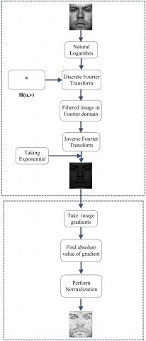
The proposed procedure to obtain illumination insensitive representation of the images, includes two steps: a) homomorphic filtering of the original image; b) further gradient face computation using the filtered image. Basically, the homomorphic filter is used to attenuate the contribution made by the low frequencies (illumination) and amplify the contribution made by high frequencies (reflectance). The net result is sharpening of features and flattening of lighting variations in an image by the simultaneous dynamic range compression and contrast enhancement. Further, the second pre-processing step, performs photometric normalization of the filtered image using the Gradient face approach. It again makes the images, illumination invariant to a greater extent.
Let Ω be an open subset of $\Re^{2}$, a scalar function h defined on Ω be the depth of the shape, and (lx, ly, lz) be the illuminant direction vector. According to Lambertian reflectance model, the image irradiance equation of the surface illuminated by a single distant light source and in the absence of self shadowing, is written as:
$I(x, y)=R(x, y) L(x, y)$ (9)
where, R(x, y) and L(x,y)=(lx, ly, lz)are the reflectance and illuminance at a pixel point (x, y) of an image whose intensity value is I(x, y) at that particular pixel.
The illumination component of an image generally tends to vary slowly by spatial variations, where as the reflectance component changes precipitously. These characteristics lead to apply Fourier transform to the image, so as to associate the low frequencies with illumination and the high frequencies with reflectance. To reduce the impact of illumination, a homomorphic filter H(u, v) is used in our proposed algorithm. It is a slightly modified form of the Gaussian high pass filter [36]. The function H(u, v) is defined as:
$H(u, v)=\left(\gamma_{H-} \gamma_{L}\right)\left[1-e^{-c\left[\frac{D^{2}(u, v)}{D_{0}^{2}}\right]}\right]+\gamma_{L}$ (10)
where, D(u, v) is the distance from a point (u, v) in the frequency domain to the center of the frequency window. D0 is the cutoff distance measured from the origin. The parameters of the filter, γL<1 and γH>1 are chosen so as to amplify the effect of reflectance and to attenuate the effect of illumination and c is a constant to control the sharpness of the slope of the filter function as it transitions between γH and γL.
Now, take the natural logarithm of Eq. (9), as the Fourier transform of a product is not the product of transforms. Also add 1 to the original image to avoid ambiguity in considering logarithm of the image having zero intensity values. Suppose, we define
$I_{1}(x, y)=\ln (I(x, y))=\ln R(x, y)+\ln L(x, y)$ (11)
Then, after taking Fourier transform of Eq. (11)
$\mathcal{F}\left\{I_{1}(x, y)\right\}=\mathcal{F}\{\ln R(x, y)\}+\mathcal{F}\{\ln L(x, y)\}$
$\overline{\mathrm{I}_{1}(\mathrm{u}, \mathrm{v})}=\overline{R(u, v)}+\overline{L(u, v)}$ (12)
Afterwards, apply filter H(u, v), defined in Eq. (10), on $\mathrm{I}_{1}(\mathrm{u}, \mathrm{v})$, we get
$\mathrm{Z}(\mathrm{u}, \mathrm{v})=\mathrm{H}(\mathrm{u}, \mathrm{v}) \overline{\mathrm{I}_{1}(\mathrm{x}, \mathrm{y})}$ (13)
Then, taking the inverse Fourier transform of the filtered image, we obtain
$z(x, y)=\mathcal{F}^{-1}\{Z(u, v)\}$ (14)
Finally, we take the exponential of the filtered image in spatial domain in reverse order as z(x, y) was processed after taking the natural algorithm of the original image I(x, y).
$I^{\text {new }}(x, y)=e^{z(x, y)}$ (15)
Finally, we get homomorphic filtered image as Inew(x, y), which is further processed to neglect illumination effects upto a great extent. As we have discussed earlier, the value of L(x, y) depends upon the lighting source, therefore it is assumed that L(x, y) varies very slowly as compared to R(x, y). Let (i, j) be the position of any pixel in the considered image under varying illumination. Then Li,j and Li+1,j are approximately equal, where (i, j) and (i+1, j) are neighbouring points of an image. Again we consider the obtained filtered image as a function of illumination L1(x, y) and reflectance R1(x, y).
$I^{\text {new}}(x, y)=R^{1}(x, y) L^{1}(x, y)$ (16)
The filtered images are further processed in the gradient domain, so as to set up relationship with the neighbouring pixels also. The image gradients are evaluated using central difference operator in the interior of the image grid and appropriate forward and backward difference operator on the boundaries of the image. The formulae for calculating the image gradients are given as:
$p_{i, j}=\left\{\begin{array}{ll}\frac{I_{i+1, j}^{n e w}-I_{i-1, j}^{n e w}}{2} & \text { if }(i, j) \in \text { image interior } \\ I_{i+1, j}^{n e w}-I_{i, j}^{n e w} & \text { if }(i, j) \in \text { left boundary } \\ I_{i, j}^{\text {new }}-I_{i-1, j}^{\text {new }} & \text { if }(i, j) \in \text { right boundary }\end{array}\right.$
$q_{i, j}=\left\{\begin{array}{l}\frac{I_{i, j+1}^{n e w}-I_{i, j-1}^{n e w}}{2} \text { if }(i, j) \in \text { image interior } \\ I_{i, j+1}^{n e w}-I_{i, j}^{n e w} \text { if }(i, j) \in \text { upper boundary } \\ I_{i, j}^{n e w}-I_{i, j-1}^{n e w} \text { if }(i, j) \in \text { lower boundary }\end{array}\right.$
Using the above formulae of pi,j and qi,j in reflectance model defined in Eq. (16), we have
$p_{i, j}=\left(\frac{\partial R^{1}}{\partial x}\right)_{i, j} L_{i, j}^{1}$ (17)
$q_{i, j}=\left(\frac{\partial R^{1}}{\partial y}\right)_{i, j} L_{i, j}^{1}$ (18)
The absolute value of the gradient of the image Inew(x, y) is evaluated by taking the square root of the sum of the square of gradient of the image in x-direction and y-direction.
$\left|\nabla I^{n e w}(x, y)\right|=\sqrt{\left(p_{i, j}\right)^{2}+\left(q_{i, j}\right)^{2}}$$=\sqrt{\left(\left(\frac{\partial R^{1}}{\partial x}\right)_{i, j}\right)^{2}+\left(\left(\frac{\partial R^{1}}{\partial y}\right)_{i, j}\right)^{2}} \cdot L_{i, j}^{1}$ (19)
In order to attain illumination insensitive normalized image, the ratio of the absolute value of the gradient of the image to the original image intensity is computed in the following manner.
$\frac{\left|\nabla I^{n e w}(x, y)\right|}{I^{n e w}(x, y)}=\frac{\sqrt{\left(\left(\frac{\partial R^{1}}{\partial x}\right)_{i, j}\right)^{2}+\left(\left(\frac{\partial R^{1}}{\partial y}\right)_{i, j}\right)^{2}}}{R_{i, j}^{1}}$ (20)
Since the reflectance component R1(x, y) is illumination insensitive and the right hand side of Eq. (20) is independent of the illumination component L1(x, y), we have obtained illumination insensitive normalized image. In practical applications, the zero intensity value of the image in Eq. (20) gives infinite value to the illumination invariant measure. To avoid this type of ambiguity, we take the tangent inverse of the Eq. (20).
$I_{\text {final}}(x, y)=\tan ^{-1}\left(\frac{\left|\nabla I^{\text {new}}(x, y)\right|}{I^{\text {new}}(x, y)}\right)$ (21)
Figure 1. Concept map to generate illumination insensitive normalized images
Figure 2. Illumination sensitive images (Top-row), homomorphic filtered images (Middle-row), and gradient-based illumination insensitive normalized images (Last-row)
To avoid the computational difficulty for the pixels having zero value in Inew(x, y) as well as in their gradients, we set the intensity of these pixels by zero in the new Image Ifinal(x, y). The concept map of the whole process to generate illumination insensitive normalized images is given in Figure 1.
Some samples of the illumination insensitive normalized images from the Yale B database are shown in Figure 2 using the proposed algorithm.
3.2 Dimensionality reduction and matching
After getting the illumination insensitive normalized images, LSDA has been employed on the vector form of an image using the procedure explained in section 2.1. LSDA computes a projection matrix using training images along with their predefined class label information. Such a projection matrix projects the images into a low dimensional space where the images sharing same class label are closer and the images having different class label are far apart. This projection matrix is preserved for recognition phase. To identify the class of a probe image, the illumination insensitive normalized image is obtained first. This preprocessed image is projected into the same low dimensional space computed using gallery images (preserved previously). Finally, a nearest neighbourhood classifier is used to compute matching scores between probe image and gallery images. Euclidean distance measure is used as distance metric.
The proposed algorithm is tested on facial image databases with illumination artifacts. The performance of any face identification system is unfavorably affected by alterations in the facial look caused by variation in lighting. So we proposed an algorithm to preprocess the face images and to make them illumination insensitive before classify them through LSDA.
In our experimental study, we have chosen input images from standard benchmark datasets such as AR database [37], Yale, and extended Yale B database [38-41]. The results obtained using the proposed algorithm have been compared with well known state-of-art algorithms such as principal component analysis (PCA), linear discriminant analysis (LDA), local binary pattern (LBP) and local binary pattern (LBP) block-wise, with and without insensitive illumination representation.
In the first step, the facial images severely affected by illumination variation are preprocessed. An illumination insensitive normalized image representation is obtained using the procedure explained in Section 3.1. Secondly, a feature vector with a reduced dimension is obtained using LSDA. An image matrix of size n×m is converted into a vector of size nm×1, as LSDA works on vector form of data. Finally, the nearest neighbourhood classifier is used to compute matching scores between probe image and gallery images. The Euclidean distance measure is used as a distance metric.
4.1 Accuracy analysis
AR database contains facial images from 126 individuals (70 men and 56 women). All the 26 images per individual were acquired in two sessions at an interval of 2 weeks. During each session, 13 images per individual with varying facial expressions, illumination, and occlusion (sun, glasses, and scarf) were captured. It is a color image database, which is converted to a database of 256 grayscale images for experimentation. Here, we have used, in total, 100 individuals who have complete face sequences from both sessions. We select the training images and the testing images from the non-occluded face images in this dataset. In this way, we are using 14 images per subject for experiment purposes. Yale database contains 165 grayscale images of 15 individuals. There are 11 images per subject, one per different facial expression or configuration: center-light, with glasses, happy, left-light, without glasses, healthy, right-light, sad, sleepy, surprised, and wink. The extended Yale B face database contains 22230 images of 38 individuals. There are 9×65 images per person, 9 poses and 65illumination conditions (64 illumination + 1 ambient). Out of 9 poses only frontalpose and 64 illumination conditions are considered for all 38 individuals for experimentation in this paper.
The results on AR database without illumination insensitive representation are given in Table 1. The results are taken on increasing gallery size (Tr) starting from 2 images per individual to 10 images per individual. The remaining images out of14 per individual are taken as probe images (Ts). The results are taken using LBP uniform, LDA, PCA, LBP uniform blockwise and LSDA. Results are found improving with increasing gallery size. Results on illumination insensitive normalized images are listed in Table 2.
Table 1. Mean classification accuracy along with standard deviation (Mean (SD)) for AR database without illumination insensitive normalization
|
Feature Extraction |
Tr=2 Ts=12 |
Tr=4 Ts=10 |
Tr=6 Ts=8 |
Tr=8 Ts=6 |
Tr=10 Ts=4 |
Tr=12 Tr=2 |
|
LBP |
24.83 (1.72) |
32.30 (1.82) |
41.13 (1.78) |
46.67 (1.89) |
47.50 (1.17) |
48.25 (1.25) |
|
LBP- Blockwise |
47.12 (2.01) |
65.54 (1.49) |
72.56 (1.39) |
78.56 (1.34) |
84.89 (1.15) |
87.84 (1.23) |
|
LDA |
58.16 (1.58) |
74.50 (2.10) |
88.88 (2.05) |
93.08 (1.27) |
94.23 (1.65) |
97.00 (1.54) |
|
PCA |
31.52 (1.31) |
64.70 (1.38) |
77.37 (1.98) |
84.83 (1.52) |
87.00 (1.16) |
92.00 (1.22) |
|
LSDA |
81.92 (1.32) |
92.20 (1.87) |
94.50 (1.89) |
95.83 (0.72) |
97.25 (0.82) |
98.00 (0.79) |
Table 2. Mean classification accuracy along with standard deviation (Mean (SD)) for AR database after illumination insensitive normalization
|
Feature Extraction |
Tr=2 Ts=12 |
Tr=4 Ts=10 |
Tr=6 Ts=8 |
Tr=8 Ts=6 |
Tr=10 Ts=4 |
Tr=12 Ts=2 |
|
LBP |
25.73 (1.65) |
33.80 (1.78) |
42.28 (1.79) |
47.87 (1.82) |
48.52 (1.27) |
48.95 (1.26) |
|
LBP- Blockwise |
49.97 (1.45) |
67.34 (1.62) |
74.67 (1.63) |
80.23 (1.26) |
86.67 (0.75) |
89.87 (0.67) |
|
LDA |
61.00 (1.51) |
86.90 (1.58) |
92.75 (1.39) |
94.50 (1.12) |
96.13 (0.86) |
97.50 (0.83) |
|
PCA |
45.25 (1.23) |
66.00 (1.18) |
78.50 (1.54) |
86.67 (1.09) |
93.50 (1.07) |
94.75 (1.04) |
|
LSDA |
83.17 (1.52) |
92.90 (1.29) |
95.27 (1.32) |
96.83 (0.87) |
98.50 (0.65) |
99.01 (0.64) |
Table 3. Mean classification accuracy along with standard deviation (Mean (SD)) for Yale database without illumination insensitive normalization
|
Feature Extraction |
Tr=5 Ts=6 |
Tr=6 Ts=5 |
Tr=7 Ts=4 |
Tr=8 Ts=3 |
Tr=9 Ts=2 |
|
LBP |
47.11 (1.11) |
55.19 (1.23) |
56.12 (1.66) |
57.19 (1.56) |
63.23 (1.79) |
|
LBP- Blockwise |
61.11 (1.11) |
67.17 (1.19) |
71.11 (1.11) |
72.81 (1.34) |
77.67 (1.45) |
|
LDA |
81.06 (1.11) |
84.06 (1.90) |
86.13 (1.49) |
90.97 (2.01) |
92.03 (1.69) |
|
PCA |
65.91 (1.99) |
68.41 (1.91) |
76.13 (1.69) |
77.61 (2.01) |
80.21 (1.39) |
|
LSDA |
81.11 (1.09) |
84.10 (1.34) |
88.24 (1.42) |
91.51 (1.42) |
93.23 (1.82) |
Table 4. Mean classification accuracy along with standard deviation (Mean (SD)) for Yale database after illumination insensitive normalization
|
Feature Extraction |
Tr=5 Ts=6 |
Tr=6 Ts=5 |
Tr=7 Ts=4 |
Tr=8 Ts=3 |
Tr=9 Ts=2 |
|
LBP |
51.15 (1.23) |
57.69 (1.11) |
58.39 (1.39) |
61.49 (1.59) |
66.62 (1.89) |
|
LBP- Blockwise |
73.48 (1.81) |
74.77 (1.79) |
75.76 (1.39) |
76.66 (1.78) |
79.01 (1.85) |
|
LDA |
82.16 (2.01) |
85.66 (1.67) |
87.23 (1.39) |
91.07 (1.71) |
93.13(1.79) |
|
PCA |
59.31 (1.34) |
59.21 (1.45) |
61.16 (1.23) |
64.21 (2.11) |
71.11 (1.19) |
|
LSDA |
83.51 (1.59) |
85.70 (1.54) |
87.44 (1.62) |
92.11 (1.38) |
93.21 (1.42) |
Table 5. Mean classification accuracy along with standard deviation (Mean (SD)) for extended Yale B database without illumination insensitive normalization
|
Feature Extraction |
Tr=4 Ts=60 |
Tr=9 Ts=55 |
Tr=14 Ts=50 |
Tr=19 Ts=45 |
Tr=24 Ts=40 |
Tr=29 Ts=35 |
|
LBP |
11.13 (1.34) |
17.34 (1.23) |
19.82 (1.23) |
21.10 (1.11) |
22.13 (1.34) |
23.82 (1.82) |
|
LBP- Blockwise |
67.66 (1.53) |
69.67 (1.69) |
73.16 (1.46) |
74.11 (1.59) |
79.11 (1.55) |
81.51 (1.25) |
|
LDA |
53.56 (1.61) |
76.86 (2.90) |
83.23 (1.12) |
84.27 (2.10) |
85.63 (1.19) |
87.01 (1.01) |
|
PCA |
74.90 (1.29) |
77.42 (1.46) |
79.33 (1.39) |
81.71 (2.12) |
82.41 (1.50) |
85.13 (1.10) |
|
LSDA |
54.38 (1.29) |
83.20 (1.89) |
84.14 (2.02) |
85.39 (1.92) |
86.03 (1.72) |
87.33 (2.20) |
Table 6. Mean classification accuracy along with standard deviation (Mean (SD)) for extended Yale B database after illumination insensitive normalization
|
Feature Extraction |
Tr=4 Ts=60 |
Tr=9 Ts=55 |
Tr=14 Ts=50 |
Tr=19 Ts=45 |
Tr=24 Ts=40 |
Tr=29 Ts=35 |
|
LBP |
18.98 (1.89) |
25.89 (1.66) |
30.82 (1.99) |
32.30 (1.78) |
33.85 (1.58) |
34.71 (1.78) |
|
LBP- Blockwise |
75.76 (2.13) |
76.47 (1.29) |
79.06 (1.73) |
80.41 (1.39) |
80.23 (1.45) |
82.11 (1.55) |
|
LDA |
78.64 (1.62) |
96.75 (1.20) |
98.13 (1.32) |
98.83 (1.11) |
99.13 (0.43) |
99.37 (0.21) |
|
PCA |
76.40 (1.27) |
91.15 (1.49) |
96.57 (1.67) |
95.77 (1.92) |
97.18 (1.39) |
98.50 (1.23) |
|
LSDA |
96.71 (1.29) |
98.75 (1.49) |
98.94 (1.01) |
99.39 (0.12) |
99.60 (0.33) |
99.77 (0.20) |
Results on Yale database are listed in Table 3. Results are taken on increasing gallery size starting from 5 images per individual to 9 images per individual. Testing is done on the remaining images out of 11 images per individual. The results on illumination insensitive normalized images of Yale database are listed in Table 4.
The results on extended Yale B database are listed in Table 5. The results are taken on increasing gallery size starting from 4 images per individual to 29 images per individual with an interval of 5. The remaining images out of 64 images are used as probe images. The results after illumination insensitive normalization are listed in Table 6.
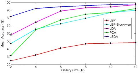
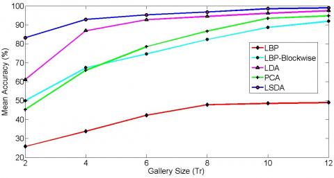
The AR database has a sufficient amount of illumination variation. Also, there is a presence of facial expressions and occlusions in the database. Overall the AR database is challenging. LSDA gives better results as compared to other algorithms. After illumination insensitive normalization, there is more improvement in the recognition rate. The recognition rate approaches up to 99% using LSDA after images being illumination insensitive normalized. In the case of small gallery size, LBP, LBP blockwise, PCA, and LDA do not give a significant recognition rate, whereas LSDA gives a reasonable recognition rate at small gallery size also (see Table 1, Table 2). It can also be justified by giving a glance at the graphical representation of mean accuracy versus the number of training images in Figure 3.
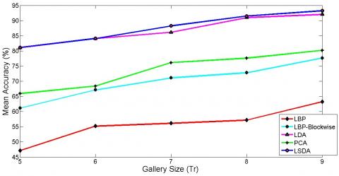
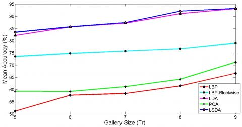
Yale database contains moderate illumination variation, expression variation, and pose variation. Yale database is a tough database; near 100% recognition is difficult. All the algorithms give slight improvements in recognition rate after illumination insensitive normalization, but LSDA outperforms others. Even LDA gives quite similar results to LSDA. The graphical representation of mean accuracy versus the number of training images is given in Figure 4 for the Yale database.
(a) Without illumination insensitive normalization
(b) After illumination insensitive normalization
Figure 3. Mean classification accuracy for AR database
(a) Without illumination insensitive normalization
(b) After illumination insensitive normalization
Figure 4. Mean classification accuracy for Yale database
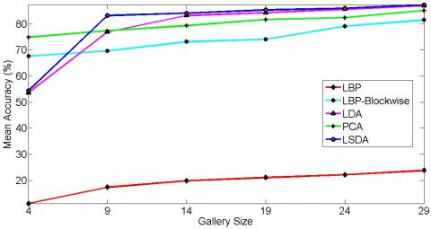
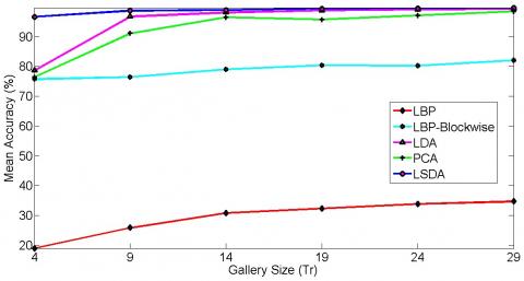
Extended Yale database B is severely affected by illumination variation. Experiments are conducted for single pose and 64 illumination conditions to investigate the real output of the proposed illumination insensitive normalization approach. There is a significant improvement in the recognition rate after illumination insensitive normalization using each algorithm tested. Results obtained by LDA are close to LSDA. Still, LSDA outperforms LDA. The recognition result without illumination insensitive normalization approaches up to 90%, whereas after illumination insensitive normalization, the recognition rate approaches up to 100%. So there is an improvement of up to 10%. It can also be justified by giving a glance at the graphical representation of mean accuracy versus the number of training images in Figure 5.
(a) Without illumination insensitive normalization
(b) After illumination insensitive normalization
Figure 5. Mean classification accuracy for extended Yale B database
For comparison, we also tested our preprocessing approach to make the images illumination insensitive, with existing illumination normalization methods provided by Wang et al. [7] and Tan et al. [22]. For experimentation, half of the images per individual, in each dataset have been treated as training images and rest half of the images as test images. All the results for mean accuracies with three datasets are given in Table 7.
Table 7. Comparison of illumination insensitive techniques
|
Dataset |
Weberfaces [7] |
Processed faces [22] |
Proposed approach |
|
AR |
90.15% |
91.97% |
96.00% |
|
Yale |
80.25% |
81.33% |
85.70% |
|
Extended YaleB |
92.75% |
99.84% |
99.94% |
A detailed statistical analysis has been performed to analyse the performance of the results obtained with the proposed algorithm. This analysis shows that LSDA is significantly better than other algorithms for illumination insensitive normalized images. To carry out statistical analysis, two tailed F-test and two tailed t-test have been performed. The values of mean accuracy and standard deviation, used for these tests are listed in Table 2, Table 4 and Table 6.
4.2.1 F-test
Two tailed F-test with equal variances has been performed at 5% level of significance for testing the equality of variances of the results with the two pairs of algorithms. The calculated value of F-statistics has been given in the Table 8, Table 9 and Table 10 for the datasets AR, Yale and extended Yale B respectively. It has been observed that the hypothesis of equal variances is accepted for all the datasets as all the calculated F values are in the range of two tailed F critical values except for few cases in AR and extended Yale B database. The hypothesis of equal variances is rejected in these cases as variance of LSDA is comparatively less as compare to LDA and PCA.
Table 8. Statistical analysis (F-test) for the proposed algorithm and other algorithms for AR database
|
Tr |
Comparison of LSDA and LDA |
Comparison of LSDA and PCA |
||||
|
H |
F-statistic |
DOF |
H |
F-ststistic |
DOF |
|
|
2 |
0 |
1.0133 |
(49,49) |
0 |
1.5271 |
(49,49) |
|
4 |
0 |
0.6666 |
(49,49) |
0 |
1.1951 |
(49,49) |
|
6 |
0 |
0.9018 |
(49,49) |
0 |
0.7347 |
(49,49) |
|
8 |
0 |
0.6034 |
(49,49) |
0 |
0.6371 |
(49,49) |
|
10 |
0 |
0.5713 |
(49,49) |
1 |
0.3690 |
(49,49) |
|
12 |
0 |
0.5946 |
(49,49) |
1 |
0.3787 |
(49,49) |
|
F-critical=(0.5674,1.7622) |
||||||
Table 9. Statistical analysis (F-test) for the proposed algorithm and other algorithms for Yale database
|
Tr |
Comparison of LSDA and LDA |
Comparison of LSDA and PCA |
||||
|
H |
F-statistic |
DOF |
H |
F-ststistic |
DOF |
|
|
5 |
0 |
0.6258 |
(49,49) |
0 |
1.7717 |
(49,49) |
|
6 |
0 |
0.8504 |
(49,49) |
0 |
0.7402 |
(49,49) |
|
7 |
0 |
1.3583 |
(49,49) |
0 |
1.3583 |
(49,49) |
|
8 |
0 |
0.6513 |
(49,49) |
0 |
0.6011 |
(49,49) |
|
9 |
0 |
0.6293 |
(49,49) |
0 |
0.5892 |
(49,49) |
|
F-critical=(0.5674,1.7622) |
||||||
Table 10. Statistical analysis (F-test) for the proposed algorithm and other algorithms for Extended Yale B database
|
Tr |
Comparison of LSDA and LDA |
Comparison of LSDA and PCA |
||||
|
H |
F-statistic |
DOF |
H |
F-ststistic |
DOF |
|
|
4 |
0 |
0.6341 |
(49,49) |
0 |
1.0317 |
(49,49) |
|
9 |
0 |
1.5417 |
(49,49) |
0 |
1 |
(49,49) |
|
14 |
0 |
0.5855 |
(49,49) |
1 |
0.3658 |
(49,49) |
|
19 |
1 |
0.0117 |
(49,49) |
1 |
0.0039 |
(49,49) |
|
24 |
0 |
0.5890 |
(49,49) |
1 |
0.0564 |
(49,49) |
|
29 |
0 |
0.9070 |
(49,49) |
1 |
0.0264 |
(49,49) |
|
F-critical=(0.5674,1.7622) |
||||||
4.2.2 t-test
Two tailed t-test with equal means has been performed at 5% level of significance for testing the equality of means of the results with the two pairs of algorithms. Those two algorithms are chosen whose mean accuracy is somewhat close to the mean accuracy of LSDA as seen by the graphs in Figure 3 (b), Figure 4 (b) and Figure 5 (b). Here we assume equal variances of the results with two considered algorithms, so pooled variance is calculated to find the value of t-statistic. The calculated values oft-statistics have been given in the Table 11, Table 12 and Table 13 for the datasets AR, Yale, extended Yale B respectively. It has been observed that the hypothesis of equal means is rejected for all the datasets as all the calculated t values are greater than t-critical value except in few cases for Yale database. So we can say that both LSDA and LDA are comparable algorithms for Yale database, whereas LSDA outperforms LBP-blockwise for the same database. It has been concluded from t-test that mean accuracy is improved using LSDA for AR and extended Yale B database.
Table 11. Statistical analysis (t-test) for the proposed algorithm and other algorithms for AR database
|
Tr |
Comparison of LSDA and LDA |
Comparison of LSDA and PCA |
||||
|
H |
t-statistic |
$S_{p}^{2}$ |
H |
t-ststistic |
$S_{p}^{2}$ |
|
|
2 |
1 |
73.1679 |
2.2952 |
1 |
137.1305 |
1.9116 |
|
4 |
1 |
20.8000 |
2.0803 |
1 |
108.7990 |
1.5283 |
|
6 |
1 |
9.2958 |
1.8373 |
1 |
58.4636 |
2.0570 |
|
8 |
1 |
11.6172 |
1.0056 |
1 |
51.5132 |
0.9725 |
|
10 |
1 |
15.5457 |
0.5810 |
1 |
28.2400 |
0.7837 |
|
12 |
1 |
10.1874 |
0.5493 |
1 |
24.6676 |
0.7456 |
|
Degrees of freedom (DOF) = 98; $S_{p}^{2}$ =pooled variance; t-critical=1.9845 |
||||||
Table 12. Statistical analysis (t-test) for the proposed algorithm and other algorithms for Yale database
|
Tr |
Comparison of LSDA and LDA |
Comparison of LSDA and PCA |
||||
|
H |
t-statistic |
$S_{p}^{2}$ |
H |
t-ststistic |
$S_{p}^{2}$ |
|
|
5 |
1 |
3.7247 |
3.2841 |
1 |
29.4384 |
2.9021 |
|
6 |
0 |
0.1245 |
2.5802 |
1 |
32.7307 |
2.7879 |
|
7 |
0 |
0.6959 |
2.2783 |
1 |
38.6912 |
2.2783 |
|
8 |
1 |
3.3467 |
2.4142 |
1 |
48.5053 |
2.5364 |
|
9 |
0 |
0.2476 |
2.6103 |
1 |
43.0544 |
2.7195 |
|
Degrees of freedom (DOF) = 98; $S_{p}^{2}$ =pooled variance; t-critical=1.9845 |
||||||
Table 13. Statistical analysis (t-test) for the proposed algorithm and other algorithms for extended Yale B database
|
Tr |
Comparison of LSDA and LDA |
Comparison of LSDA and PCA |
||||
|
H |
t-statistic |
$S_{p}^{2}$ |
H |
t-ststistic |
$S_{p}^{2}$ |
|
|
4 |
1 |
61.7008 |
2.1443 |
1 |
79.3335 |
1.6385 |
|
9 |
1 |
7.3921 |
1.8301 |
1 |
25.5034 |
2.2010 |
|
14 |
1 |
3.4460 |
1.3812 |
1 |
8.5867 |
1.9045 |
|
19 |
1 |
3.5467 |
0.6233 |
1 |
13.3059 |
1.8504 |
|
24 |
1 |
6.1314 |
0.1469 |
1 |
11.9778 |
1.0205 |
|
29 |
1 |
9.7532 |
0.0421 |
1 |
7.2064 |
0.7764 |
|
Degrees of freedom (DOF) = 98; $S_{p}^{2}$=pooled variance; t-critical=1.9845 |
||||||
A technique using a gradient data of the image has been proposed to obtain an insensitive illumination representation of the image. The application of insensitive illumination representation has been investigated in the context of face recognition and found very useful. The proposed algorithm is validated on various databases containing slightest to severe illumination variation and is found very effective on databases containing severe illumination variation. Five algorithms are tested, LBP, LBP-blockwise, PCA, LDA and LSDA. Even though all algorithms give slight improvement but LDA and LSDA are found more promising with illumination insensitive normalization. Besides the nearest neighborhood classifier, the other classification approaches such as SVM, random forest, etc. may be used in the future work.
[1] Han, H., Shan, S., Chen, X., Gao, W. (2013). A comparative study on illumination preprocessing in face recognition. Pattern Recognition, 46(6): 1691-1699. https://doi.org/10.1016/j.patcog.2012.11.022
[2] Horn, B.K. (1974). Determining lightness from an image. Computer Graphics and Image Processing, 3(4): 277-299. https://doi.org/10.1016/0146-664X(74)90022-7
[3] Xie, X., Zheng, W., Lai, J., Yuen, P.C. (2008) Face illumination normalization on large and small scale features. 2008 IEEE Conference on Computer Vision and Pattern Recognition, Anchorage, AK, pp. 1-8. https://doi.org/10.1109/CVPR.2008.4587811
[4] Lee, P.H, Wu, S.W, Hung, Y.P. (2012). Illumination compensation using oriented local histogram equalization and its application to face recognition. IEEE Transactionson Image Processing, 21(9): 4280-4289. https://doi.org/10.1109/TIP.2012.2202670
[5] Zhang, T., Tang, Y.Y., Fang, B., Shang, Z., Liu, X. (2009). Face recognition under varying illumination using gradientfaces. IEEE Transactions on Image Processing, 18(11): 2599-2606. https://doi.org/10.1109/TIP.2009.2028255
[6] Tzimiropoulos, G., Zafeiriou, S., Pantic, M. (2012). Subspace learning from image gradient orientations. IEEE Transactions on Pattern Analysis and Machine Intelligence, 34(12): 2454-2466. https://doi.org/10.1109/TPAMI.2012.40
[7] Wang, B., Li, W., Yang, W., Liao, Q. (2011). Illumination normalization based on Weber’s law with application to face recognition. IEEE Signal Processing Letters, 18(8): 462-465. https://doi.org/10.1109/LSP.2011.2158998
[8] Ding, C., Choi, J., Tao, D., Davis, L.S. (2016). Multi-directional multi-level dual-cross patterns for robust face recognition. IEEE Transactions on Pattern Analysis and Machine Intelligence, 38(3): 518-531. https://doi.org/10.1109/TPAMI.2015.2462338
[9] Kumar, P.M., Gandhi, U., Varatharajan, R., Manogaran, G., Jidhesh, R., Vadivel, T. (2019). Intelligent face recognition and navigation system using neural learning for smart security in Internet of Things. Cluster Computing, 22: 7733-7744. https://doi.org/10.1007/s10586-017-1323-4
[10] Cai, D., He, X., Zhou, K., Han, J., Bao, H. (2007). Locality sensitive discriminant analysis. IJCAI International Joint Conference on Artificial Intelligence, pp. 708-713.
[11] Liu, J., Wang, Z., Liu, J., Feng, Z. (2008). Face recognition with locality sensitive discriminant analysis based on matrix representation. 2008 IEEE International Joint Conference on Neural Networks (IEEE World Congress on Computational Intelligence), Hong Kong, 2008, pp. 4052-4058. https://doi.org/10.1109/IJCNN.2008.4634380
[12] Chen, L.H., Yang, Y.H., Chen, C.S., Cheng, M.Y. (2011). Illumination invariant feature extraction based on natural images statistics - taking face images as an example. CVPR 2011, Providence, RI, 681-688. https://doi.org/10.1109/CVPR.2011.5995621
[13] da Cunha, A., Zhou, J., Do, M. (2006). The nonsubsampled contourlet transform: Theory, design, and applications. IEEE Transactions on Image Processing, 15(10): 3089-3101. https://doi.org/10.1109/TIP.2006.877507
[14] Xie, X., Lai, J., Zheng, W.S. (2010). Extraction of illumination invariant facial features from a single image using non subsampled contourlet transform. Pattern Recognition, 43(12): 4177-4189. https://doi.org/10.1016/j.patcog.2010.06.019
[15] Nabatchian, A., Abdel-Raheem, E., Ahmadi, M. (2011). Illumination invariant feature extraction and mutual-information-based local matching for face recognition under illumination variation and occlusion. Pattern Recognition, 44(10-11): 2576-2587. https://doi.org/10.1016/j.patcog.2011.03.012
[16] Cao, X., Shen, W., Yu, L., Wang, Y., Yang, J., Zhang, Z. (2012). Illumination invariant extraction for face recognition using neighboring wavelet coefficients. Pattern Recognition, 45(4): 1299-1305. https://doi.org/10.1016/j.patcog.2011.09.010
[17] Zhang, J., Xie, X. (2012). A study on the effective approach to illumination-invariant face recognition based on a single image. In: Zheng, W.S., Sun, Z., Wang, Y., Chen, X., Yuen, P., Lai, J. (eds) Biometric Recognition, Lecture Notes in Computer Science, 7701: 33-41. https://doi.org/10.1007/978-3-642-35136-5_5
[18] Hu, Y., Mian, A.S., Owens R. (2012). Face recognition using sparse approximated nearest points between image sets. IEEE Transactions on Pattern Analysis and Machine Intelligence, 34(10): 1992-2004. https://doi.org/10.1109/TPAMI.2011.283
[19] Naseem, I., Togneri, R., Bennamoun, M. (2010). Linear regression for face recognition. IEEE Transactions on Pattern Analysis and Machine Intelligence, 32(11): 2106-2112. https://doi.org/10.1109/TPAMI.2010.128
[20] Anvaripour, M., Ebrahimnezhad, H. (2015). Accurate object detection using local shape descriptors. Pattern Analysis and Applications, 18(2): 277-295. https://doi.org/10.1007/s10044-013-0342-x
[21] Biswas, A., Ghose, M.K. (2014). Face recognition algorithm based on orientation histogram of Hough peaks. International Journal of Artificial Intelligence & Applications, 5(5): 107-114. http://dx.doi.org/10.5121/ijaia.2014.5509
[22] Tan, X., Triggs, B. (2010). Enhanced local texture feature sets for face recognition under difficult lighting conditions. IEEE Transactions on Image Processing, 19(6): 1635-1650. https://doi.org/10.1109/TIP.2010.2042645
[23] Balaban, S. (2015) Deep learning and face recognition: the state of the art. Biometric and Surveillance Technology for Human and Activity Identification XII, 9457: 68-75. https://doi.org/10.1117/12.2181526
[24] Elmahmudi, A., Ugail, H., (2019). Deep face recognition using imperfect facial data. Future Generation Computer Systems, 99: 213-225. https://doi.org/10.1016/j.future.2019.04.025
[25] Bah, S.M., Ming, F. (2020). An improved face recognition algorithm and its application in attendance management system. Array, 5: 100014. https://doi.org/10.1016/j.array.2019.100014
[26] Jin, Y., Ruan, Q.Q., Wang, Y.Z. (2010). 3D face recognition using tensor orthogonal locality sensitive discriminant analysis. In: IEEE 10th International Conference on Signal Processing (ICSP), pp. 1394-1397. https://doi.org/10.1109/ICOSP.2010.5656910
[27] Taigman, Y., Yang, M., Ranzato, M., Wolf, L. (2014). Deepface: Closing the gap to human-level performance in face verification. 2014 IEEE Conference on Computer Vision and Pattern Recognition, Columbus, OH, pp. 1701-1708. https://doi.org/10.1109/CVPR.2014.220
[28] Benkaddour, M.K., Bounoua, A. (2017). Feature extraction and classification using deep convolutional neural networks, PCA and SVC for face recognition. Traitement du Signal, 34(1-2): 77-91. https://doi.org/10.3166/TS.34.77-91
[29] Sun, Y., Chen, Y., Wang, X., Tang, X. (2014). Deep learning face representation by joint identification verification. In: Ghahramani, Z., Welling, M., Cortes, C., Lawrence, N., Weinberger, K. (eds) Advances in Neural Information Processing Systems 27, Curran Associates, Inc., 1988-1996. https://doi.org/10.5555/2969033.2969049
[30] Ding, C., Tao, D. (2015). Robust face recognition via multimodal deep face representation. IEEE Transactions on Multimedia, 17(11): 2049-2058. https://doi.org/10.1109/TMM.2015.2477042
[31] Martinez, A., Kak, A.C. (2001). PCA versus LDA. IEEE Transactions on Pattern Analysis and Machine Intellegence, 23(2): 228-233. https://doi.org/10.1109/34.908974
[32] Zhao, W., Krishnaswamy, A., Chellappa, R., Swets, D.L., Weng, J. (1998) Discriminant analysis of principal components for face recognition. Face Recognition, Springer Berlin Heidelberg, 73-85. https://doi.org/10.1007/978-3-642-72201-1_4
[33] Etemad, K., Chellappa, R. (1997). Discriminant analysis for recognition of human face images. Optical Society of America, 14(8): 1724-1733. https://doi.org/10.1007/BFb0015988
[34] Moon, H, Phillips, P (2001) Computational and performance based aspects of PCA based face recognition algorithms. Perception, 30(3): 303-321. https://doi.org/10.1068/p2896
[35] Draper, B.A., Baek, K., Bartlett, M.S., Beveridge, J. (2003). Recognizing faces with PCA and ICA. Computer Vision and Image Understanding, 91: 115-137. https://doi.org/10.1016/S1077-3142(03)00077-8
[36] Gonzalez, R. (2009). Digital Image Processing. Pearson Education.
[37] Martinez, A.M., Benavente, R. (1998). The AR face database. CVC Technical Report.
[38] Georghiades, A.S., Belhumeur, P.N., Kriegman, D.J. (2001). From few to many: Illumination cone models for face recognition under variable lighting and pose. IEEE Transactions on Pattern Analysis and Machine Intelligence, 23(6): 643-660. https://doi.org/10.1109/34.927464
[39] Lee, K.C., Ho, J., Kriegman, D.J. (2005). Acquiring linear subspaces for face recognition under variable lighting. Transactions on Pattern Analysis and Machine Intelligence, 27(5): 684-698. https://doi.org/10.1109/TPAMI.2005.92
[40] Liu, H.D., Yang, M., Gao, Y., Cui, C. (2014). Local histogram specification for face recognition under varying lighting conditions. Image and Vision Computing, 32(5): 335-347. https://doi.org/10.1016/j.imavis.2014.02.010
[41] Saini, N., Sinha, A. (2015). Face and palm print multimodal biometric systems using Gabor-Wigner transform as feature extraction. Pattern Analysis and Applications, 18(4): 921-932. https://doi.org/10.1007/s10044-014-0414-6