Na Jiang* | Jiyuan Li
© 2020 IIETA. This article is published by IIETA and is licensed under the CC BY 4.0 license (http://creativecommons.org/licenses/by/4.0/).
OPEN ACCESS
Traditional semantic segmentation methods cannot accurately classify high-resolution remote sensing images, due to the difficulty in acquiring the correlations between geophysical objects in these images. To solve the problem, this paper proposes an improved semantic segmentation method for remote sensing images based on neural network. Based on residual network, the proposed algorithm changes the dilated convolution kernels in the dilated spatial pyramid pooling (SPP) module before extracting the correlations between geophysical objects, thus improving the accuracy of segmentation. Next, the high resolution of the input image was maintained through deconvolution, and the semantic segmentation was realized by the pixel-level method. To enhance the robustness of our algorithm, the dataset was expanded through random cropping and stitching of images. Finally, our algorithm was trained and tested on the Potsdam dataset provided by the International Society for Photogrammetry and Remote Sensing (ISPRS). The results show that our algorithm was 1.4% more accurate than the DeepLab v3 Plus. The research results shed new light on the semantic segmentation of high-resolution remote sensing images.
remote sensing images, pixel-level method, residual network (ResNet), dilated spatial pyramid pooling (SPP), sub-pixel up-sampling, semantic segmentation
With the rapid development of satellite sensors, the resolution of remote sensing images has been improved continuously. High-resolution remote sensing images provide the refined information that is applicable to various tasks of earth observation, which benefit many aspects of society and economy. Meanwhile, the refined information also poses new challenges to the intelligent interpretation of high-resolution remote sensing images.
The key to interpreting high-resolution remote sensing images lies in semantic segmentation. However, the interpretation requires the processing of massive information on geophysical observations. Due to the sheer amount of data, manual classification would be inaccurate, time-consuming, and labor-intensive. Similarly, traditional image segmentation methods cannot effectively handle the big data of remote sensing images. Based on the underlying features, the traditional methods have poor robustness and low recognition accuracy.
Against this backdrop, automatic semantic segmentation methods, namely, deep convolutional neural network (D-CNN), has attracted widespread attention. Many typical CNNs have been successfully designed to semantically segment multiple objects, namely, fully-connected network (FCN) [1], SegNet [2], pyramid scene parsing network (PSPNet) [3], DeepLab [4], and deconvolution network. In general, CNN-based semantic segmentation methods can be divided into block-level methods and pixel-level methods. The block-level methods classify each pixel in the input image by sliding every small image block. Such methods take a long time to classify the entire image, and have strict requirements on the block size of the input image. The pixel-level methods provide an end-to-end architecture, capable of maintaining the global content structure of the input image. For example, the FCN can effectively classify input images of any size.
Because geophysical features vary greatly in size, the segmentation method for high-resolution remote sensing images should recognize the features of small geophysical objects, as well as the global features of large geophysical background. In recent years, deep learning (DL) has become a hot topic among researchers engaging in semantic segmentation [5-9]. For example, the FCN and its improved versions have optimized the semantic segmentation of multiple datasets, such as Pascal VOC [10] and Cityscapes [11]. However, there are two problems in the application of deep neural networks (DNNs) in the segmentation of high-resolution remote sensing images. On the one hand, the DNNs may suffer from over-fitting facing the imbalance of different geophysical features, which arises from the diversity of geophysical information and the imbalance between information classes. On the other hand, the loss of local informaiton may occur due to the up-sampling after DNN feature extraction.
To solve the two problems, this paper proposes an improved semantic segmentation algorithm for remote sensing images based on neural network (NN). The proposed algorithm, as a pixel-level method extended from ResNet101, extracts the correlations between geophysical objects by changing the dilated convolution kernels in the dilated spatial pyramid pooling (SPP) module. On this basis, the high-resolution remote sensing image was segmented into multiple geophysical objects at a reasonable precision. The segmentation effect of our algorithm was verified on the Potsdam dataset provided by International Society for Photogrammetry and Remote Sensing (ISPRS) [12].
The remainder of this paper is organized as follows: Section 2 compares the relevant semantic segmentation methods; Section 3 details the proposed algorithm, namely, the improved semantic segmentation algorithm for remote sensing images; Section 4 experimentally verifies the proposed algorithm; Section 5 analyzes the experimental results; Section 6 puts forward the conclusions.
2.1 Semantic segmentation of high-resolution remote sensing images
Remote sensing images of contain numerous complex objects in various sizes. It is immensely difficult to segment all these objects at the same time. Improving the resolution clarifies the details of redundant objects, but adds to the difficulty in image segmentation.
In semantic segmentation, high-level and abstract features are suitable for large and easily-confused objects, while low-level and original features benefit small objects. The integration between features on different levels provides rich informaiton for semantic segmentation. Therefore, the features on different levels should be combined to extract the complex objects from remote sensing images.
In recent years, the DNNs [13] achieve excellent performance in semantic segmentation, through the combination of representation learning and classifier training. For instance, the FCN achieves end-to-end training through up-sampling and resolution matching between output feature map and input image. However, it is difficult for the FCN to acquire low-level features for accurate edge prediction, under the requirements of dense prediction.
The FCN is modified and extended into SegNet [7] and U-Net [14], using jump connections. The input image can be classified accurately at the pixel level, for the cascade structure allows the decoding layer to reuse low-level feature maps, which contain more details. Compared with U-Net, SegNet records the pool index in the encoder and reuses it in the decoder, making segmentation even more accurate. When the feature maps are of the same size, the encoder layer and the decoder layer are connected explicitly. However, some useful details about geophysical objects and image scenes are deleted, with the increase in the receptive field.
Dilated convolution widens the receptive field by expanding the convolution, without changing the number of additional parameters or the size of feature map. Thanks to dilated convolution, DeepLab and PSPNet are now widely adopted for semantic segmentation.
2.2 Residual network (ResNet)
With the growth in depth, DNNs can learn more features at the cost of longer training and slower convergence. The depth growth is impeded by vanishing gradient. If the depth continues to grow after reaching a threshold, the learning rate and accuracy will start to decline. To prevent network degradation, He et al. [6] put forward the concept of residual unit and ResNet. In the residual unit, the input and output are simply superimposed in the short-circuit connection. The simple operation suppresses network degradation, and improves the speed and effect of network training, without adding additional parameters or calculations to the network. Multiple residual units are stacked into a DNN called ResNet. Not every layer of the ResNet requires additional pooling operation.
The most representative ResNets include ResNet56, ResNet101 and ResNet152. The figures stand for the number of layers in the ResNets. The ResNets have four typical features: (1) The small size of the network controls the number of parameters; (2) The number of feature maps increases layer by layer, ensuring the expression of output features; (3) The propagation efficiency is improved by adopting many down-sampling operations and a few pooling layers; (4) The dropout [15] is replaced by batch normalization (BN) [16] and global average pooling for regularization, resulting in fast training. With the above advantages, the ResNet has been widely adopted for semantic segmentation of high-resolution remote sensing images.
2.3 Dilated SPP
In the CNN, the convolutional layers can handle inputs of any scale. The input image is convoluted and pooled repeatedly until reaching the fully-connected layer. Without needing cropping or scaling, SPP can convert feature maps of any size into fixed-size eigenvectors, providing fixed-size inputs required by the classifier. During semantic segmentation, SPP mainly acquires the context of the scenes and the contextual connections.
If the objects of semantic segmentation are on varied scales, the segmentation results depend heavily on long-distance contextual informaiton and informaiton of different scales. To enlarge the receptive field, a common practice is to perform SPP on the extracted feature maps, and fuse multi-scale information by jump connections. Nevertheless, the spatial resolution is reduced after each pooling, and might get lost after multiple pooling operations, which undermines the segmentation effect. Dilated convolution can enlarge the receptive field without losing information. It is possible to obtain multi-scale informaiton gain by parallel or cascade stacking dilated convolutions with different dilation rates.
2.4 Up-sampling based on sub-pixel convolution
The DNNs achieve in-depth learning of image features through multiple convolutions. During the convolution, the spatial resolution of feature maps decreases due to the repeated pooling operations. In pixel-based semantic segmentation, each pixel in the input image is given a label based on its class. For example, the images from the ISPRS Potsdam dataset and the segmentation results are shown in Figure 1. The pixels in the high-resolution remote sensing images are divided into six classes, namely, impervious layer, buildings, shrubs, trees, vehicles, and background. The six classes are respectively colored in white, blue, bluish green, green, yellow, and red.
After multiple convolutions, the size of feature map becomes smaller. The feature map should be restored to the original size for pixel-level comparison with label data. For this purpose, the sub-pixel convolution can expand the low-resolution feature map to high-resolution output. The sub-pixel convolutional layer does not use any artificially designed expansion filters, such as bilinear samplers or dual trilinear samplers. Instead, this layer learns complex expansion operations through training. In this way, the overall computing time is reduced, and the image can be reconstructed with a high accuracy.
Figure 1. The ISPRS Potsdam dataset and the segmentation results
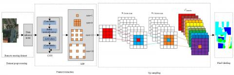
Figure 2. The overall framework of semantic segmentation of remote sensing images
3.1 Overview
In some application fields of remote sensing, the region of interest (ROI) may account for a small portion of the set of remote sensing images. In other words, the valuable image subset in the application field might be small, despite the large size of the overall set of remote sensing images.
Data enhancement is an effective way to solve the relative lack of remote sensing data. Through data enhancement, different classes of geophysical objects could be balanced, and an abundance of accurate information could be learned by expanding the dataset through DNN-based semantic segmentation (pixel labeling). Data enhancement also effectively suppresses over-fitting.
Inspired by the semantic segmentation by DeepLab, this paper adopts ResNet-based method to extract various types of geophysical features. Besides, the dilated SPP was employed to recognize geophysical details, focusing on local or global information. This is because both geophysical details and local information (i.e. geophysical features of different sizes) must be considered in the semantic segmentation of high-resolution remote sensing images.
After acquiring rich geophysical features, up-sampling should be performed to restore the feature map to the size of the input image, laying the basis for class labeling of each geophysical pixel. This paper proposes an up-sampling method for high-resolution remote sensing images based on sub-pixel convolution. In this way, high-quality up-sampling is realized at a high computing efficiency.
As shown in Figure 2, the high-resolution remote sensing data are mainly processed through four steps: data preprocessing, feature extraction (down-sampling), up-sampling, and pixel labeling. The first step (data preprocessing) generates and enhances the dataset. The second step (feature extraction) consists of two networks: the ResNet-based CNN, and the dilated SPP module. The third step (up-sampling) restores the resolution and size of the image through sub-pixel convolution. The fourth step (pixel labeling) outputs the segmentation results. (http://www2.isprs.org/commissions/comm2/wg4/potsdam-2d-semantic-labeling.html)
3.2 Data enhancement through random cropping and stitching
The set of high-resolution remote sensing images contains a large amount of data, existing as a dense cluster of various geophysical information. For a specific application, however, relatively few information and unobvious features are relevant to the accurate recognition of a type of geophysical objects. This paper enhances the limited data by randomly cropping and stitching high-resolution remote sensing images [4]. The images were randomly selected from the ISPRS Potsdam dataset [12], which offers 38 remote sensing orthoimages (resolution: 5cm; size: 6,000×6,000). Each image contains four spectra: infrared, red, green, and blue. Six types of geophysical objects are involved in the dataset, including the impervious layer (white), buildings (blue), shrubs (bluish green), trees (green), vehicles (yellow), and background (red).
The high-resolution remote sensing data were enhanced in the following steps:
Step 1. Because the graphics processing unit (GPU) has a limited memory, it is impossible to input the entire image into the network. Thus, each original RGB orthoimage (6,000×6,000) was split into 169 images (512×512) by a sliding window. The 38 original images were split into a total of 6,422 images (512×512). Let D be the dataset of the 6,422 images, and L be the set of labels corresponding to these images.
Step 2. Four images were randomly selected for enhancement from the 6,422 images. The four candidate images are denoted as $I_{k} \in D, k \in\{1,2,3,4\}$, and the set of labels corresponding to the four images are denoted as Lk, k∈{1, 2, 3, 4}.
Step 3. Each candidate image was cropped as shown in Figure 3, where Ix=512 and Iy=512 are the width and height of the 6,422 cropped images. The four candidate images in the lower part of Figure 3 were randomly chosen from the 6,422 images. For each candidate image, a random cropping point (w, h) was generated based on beta (β) distribution, and used to determine the cutting lines (yellow dashed box). The cropped areas of the four images were stitched into a new image, which is of the same size as the four images.
Mathematically, four images Ik were randomly chosen from dataset D. During each training, a cropping point (w, h) was selected from each image by random. The randomly selected cropping points obey β-distribution:
$w=\left\lfloor C_{w} I_{x}\right\rfloor, h=\left\lfloor C_{h}, I_{y}\right\rfloor$,
$C_{w} \sim \operatorname{Beta}(\beta, \beta)$,
$C_{h} \sim \operatorname{Beta}(\beta, \beta)$ (1)
where, β is a hyperparameter in training. Here, the β value is set to 0.3, which minimizes the test error [4].
Once the cropping points (w, h) were determined, the cropped areas of the four candidate images Ik were calculated, and added up to obtain the size (wk, hk) of the stitched image:
$w_{1}=w_{3}=w, w_{2}=w_{4}=I_{x}-w$,
$h_{1}=h_{2}=h, h_{3}=h_{4}=I_{y}-h$ (2)
Figure 3. The cropping of candidate images
Step 4. The cropped areas were stitched into a new image Inew, which is of the same size (512×512) as the four candidate images Ik:
$L_{n e w}=\sum_{k=1,2,3,4} R_{k} L_{k}$ (3)
where, Rk is the size ratio of the cropped area to the candidate image:
$R_{k}=\frac{w_{k} h_{k}}{I_{x} I_{y}}$ (4)
Through cropping and stitching of random images, a new training set of 6,422 images were generated based on the set of 6,422 images, which were obtained through sliding window operation over the 38 images (6,000×6,000) in the Potsdam dataset. The original dataset D and the new dataset Dm were mixed as the training set $\widetilde{D}$:
$\tilde{D}=D+D_{m}$ (5)
3.3 Feature extraction based on ResNet and SPP
There are two core issues in the extraction of geophysical features from high-resolution remote sensing images:
(1) The local features: The details of geophysical objects in high-resolution remote sensing images;
(2) The global features: The correlations between geophysical objects in high-resolution remote sensing images, i.e. the global features in the surroundings of geophysical objects on different scales.
The two issues were dealt with by a DNN based on ResNet and SPP.
3.3.1 ResNet
Thanks to the development of the DL, typical classification networks, namely, Visual Geometry Group (VGG) and ResNet, have been increasingly popular. These networks work excellently on largescale dataset like ImageNet, and support task-oriented finetuning based on training data. This paper adopts ResNet101, a typical ResNet, to extract the local features of geophysical objects:
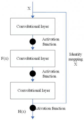
Figure 4. The residual unit
First, an identity mapping was superimposed on a stacked structure, forming a residual unit. The structure of the residual unit is illustrated in Figure 4, where x is the identity mapping inputted to the stacked structure. The identity mapping can be understood as a short-circuit connection.
Let w1, w2 and w3 be the weights of the three convolutional layers, and σ1, σ2 and σ3 be the three activation functions, respectively, in the residual unit. Then, the output F(x) of the convolutional layers can be described as:
$F(x)=w_{3} \sigma_{2}\left(w_{2} \sigma_{1}\left(w_{1} x\right)\right)$ (6)
Then, the output of the residual unit can be obtained by adding up F(x) and the identity mapping x:
$H(x)=F(x)+x$ (7)
The final output is a function of the identity mapping and the weights of convolutional layers:
$H(x)=F\left(x,\left\{w_{i}\right\}\right)+x$ (8)
Let xl and wl be the input and weight of the l-th layer, respectively. Then, the input of the l+1-th layer (i.e. the input of the l-th layer) can be expressed as:
$X_{l}+1=x_{l}+F\left(x_{l}, w_{l}\right)$ (9)
Through recursion, the feature map of the L-th layer in residual unit of any depth can be obtained as:
$X_{L}=x_{l}+\sum_{l}^{L-1} F\left(x_{l}, w_{l}\right)$ (10)
The gradient of the reverse process can be derived by the chain rule:
$\frac{\partial_{l o s s}}{\partial x_{l}}=\frac{\partial_{l o s s}}{\partial x_{L}} \cdot \frac{\partial x_{L}}{\partial x_{l}}=\frac{\partial_{l o s s}}{\partial x_{L}} \cdot\left(1+\frac{\partial}{\partial x_{L}} \sum_{i=l}^{L-1} F\left(x_{i}, W_{i}\right)\right)$ (11)
where, l is the short-circuit mechanism of the identity mapping, which can transmit the gradient without loss. This is how ResNet suppresses the vanishing gradient.
3.3.2 Dilated SPP
This paper relies on dilated SPP to extract the correlations between geophysical features. The dilated SPP is a parallel process. Each image is convoluted by multiple dilated kernels in different sizes. The multiple results are fused into an output. Dilated convolution [17, 18] increases the gap between two adjacent pixels in a kernel, without increasing the number of pixels of the kernel. Therefore, the dilated kernel is larger than the original kernel, but has the same computing cost.
In an existing dilated SPP module [19, 20], dilated kernels with four dilation rates (6, 12, 18 and 24) were used to convolute the input image, respectively, aiming to obtain the correlations between geophysical objects in difference distances to the center point. Dilated convolution enables the later convolutional layers to maintain a large feature map, without changing the number of ResNet parameters and receptive field of convolutional layer in each step. Hence, dilated convolution benefits the detection of small objects, thus improving the overall performance of the model.
As shown in Figure 5, our dilated SPP module involves four parallel dilated kernels, whose dilation rates are 1, 6, 12 and 18, respectively.
Figure 5. Our dilated SPP module
3.4 Up-sampling based on sub-pixel convolution
Each original high-resolution remote sensing image is of the size Ix×Iy×C, where C is the number of channels. The features of the original image were extracted through ResNet and dilated SPP module, yielding a feature map of the size Ix/r×Iy/r×Ck, where r is the reduction ratio, and Ck is the number of channels in the feature map.
To restore its size to the original map, the feature map was subjected to sub-pixel convolution. After convolution, the number of channels became:
$C_{s}=r^{2} \times C_{k}$ (12)
Based on the Cs output images from the sub-pixel convolution layer, the pixels at the same coordinates were stitched into r×r regions. All these regions were merged in the order of pixels into an image of the width Ix/r×r=Ix and the height Iy/r×r=Iy.
4.1 Experimental setting
To verify its effectiveness, the proposed method was verified through experiments on the Potsdam dataset, a 2D dataset provided by the ISPRS the Potsdam dataset, and compared with other labeling methods for remote sensing images. Under the TensorFlow framework, the experiments were carried out on a hardware-accelerated GPU (Nvidia GeForce GTX 1080 Ti, 11GB).
By the data enhancement method in Subsection 3.1, a total of 12,844 images (512×512×3; RGB3 channel) were obtained. The image set was divided into a training set (7,700), a verification set (2,572), and a test set (2,572) at the ratio of 6:2:2. The contrastive methods include FCN-32S, FCN-8S, U-Net, SegNet, and DeepLab v3 Plus. The effectiveness of each method was evaluated against three metrics: F1 score, average recall, and overall accuracy.
4.2 Training
During the training, the ResNet was trained based on the parameters of ResNet101. Overall, ResNet101 consists of five parts. The number of convolutions in the five parts is 2, 3×3, 3×4, 3×23, and 3×3, respectively. The parameters of ResNet101 were finetuned for the training set. The stochastic gradient descent (SGD) was adopted for the training, with cross entropy as the loss function. The maximum number of iterations was set to 30,000. Ten samples were considered as a batch. Under the polynomial decay strategy, the initial and final learning rates were set to 0.007 and 0.000001, respectively. The weight attenuation and momentum were set to 0.0002 and 0.9, respectively.
4.3 Experimental results
The F1 score, average recall, and overall accuracy of each method in the classification of the six types of geophysical objects are listed in Table 1 below.
As shown in Table 1, our method achieved much better results in four of the six types of geophysical objects. Our method (data enhancement only) was clearly more accurate than Deep Lab v3 plus in five types of geophysical objects, especially in terms of vehicles; Our method (sub-pixel up-sampling only) was clearly more accurate than Deep Lab v3 Plus in three types of geophysical objects, especially in terms of background; Our method (data enhancement + sub-pixel up-sampling) was 1.2%, 0.5%, 1.4%, and 4.2% more accurate than Deep Lab v3 Plus in terms of impervious bed, buildings, shrubs, and trees, respectively.
Next, six original images were selected, and segmented by our method. The original images, labels, and segmentation results are presented in Figure 6 below. It can be seen that our method achieved good semantic segmentation effects, with virtually no segmentation mistake.
In Figures 6(a) and 6(c), the building edges segmented by our method differed slightly from the labeled data in the black boxes. Through comparison with the original images, it is confirmed that the building edges recognized by our method are closer to the reality. In Figures 6(d) and 6(e), the vehicles recognized by our method in the black boxes are more accurate than the labeled data. In Figure 6(e), the two vehicles in the black boxes are very close to each other; the labeled data treated them as the same object, while our method treated them as separate objects. In Figures 6(d) and 6(f), the edges of trees identified by our method were close to those in the original image, but some details of the trees were lost in the labeled data.
Table 1. The experimental results
|
Model |
Impervious layer |
Buildings |
Shrubs |
Trees |
Vehicles |
Background |
F1 score |
Average recall |
Overall accuracy |
|
FCN-32S |
0.782 |
0.836 |
0.712 |
0.661 |
0.740 |
0.175 |
0.651 |
0.716 |
0.759 |
|
FCN-8S |
0.801 |
0.852 |
0.728 |
0.681 |
0.827 |
0.232 |
0.685 |
0.751 |
0.778 |
|
U-Net |
0.790 |
0.848 |
0.788 |
0.749 |
0.875 |
0.260 |
0.719 |
0.784 |
0.798 |
|
SegNet |
0.811 |
0.864 |
0.780 |
0.738 |
0.857 |
0.236 |
0.714 |
0.773 |
0.803 |
|
Deep Lab v3 Plus |
0.892 |
0.928 |
0.833 |
0.784 |
0.882 |
0.316 |
0.772 |
0.820 |
0.860 |
|
Our method (data enhancement only) |
0.897 |
0.935 |
0.844 |
0.822 |
0.902 |
0.283 |
0.785 |
0.817 |
0.871 |
|
Our method (sub-pixel up-sampling only) |
0.902 |
0.930 |
0.837 |
0.816 |
0.883 |
0.338 |
0.784 |
0.814 |
0.873 |
|
Our method (data enhancement + sub-pixel up-sampling) |
0.904 |
0.933 |
0.847 |
0.826 |
0.898 |
0.297 |
0.786 |
0.824 |
0.874 |
Figure 6. The segmentation results of our methods on six images
The experimental results show that the edges of trees recognized by our method differed from the edges in the labeled data, as shown in the black boxes of Figures 6(d) and 6(f). Comparing with the original image, it is found that the trees are mostly crowns in the remote sensing images, for the high-resolution satellite shots images from the top. The crowns vary greatly with seasons, geographic locations, and tree species. The variation is further enhanced by the lighting, weather, and other conditions at the time of image acquisition.
In the original image of Figure 6(e), the leaves are so scarce that the branches are very prominent. Even the thin branches at the ends are highly legible. However, the branches cannot be easily recognized by the naked eye, due to the small contrast between branches and the background. That is why these geophysical objects are not accurately labeled. This is a typical problem in the object recognition of high-resolution remote sensing images. Probing into this problem helps to improve the accuracy of semantic segmentation of high-resolution remote sensing images.
Moreover, our method was more accurate than the labeled data in recognizing the details of vehicles in all images that contain vehicle(s). Take Figure 6(e) for example. Our method clearly distinguished between the small vehicles that are close to each other. For objects like vehicles, planes, and ships, geometric details are critical to their classification and model identification. However, the labels of the vehicles in Figure 6(e) are basically straight lines, failing to reflect the local details of the vehicles. Of course, this is not the labeler’s fault. Even if the naked eye can recognize the shape changes of the vehicles, it is too costly to label all these details manually.
Currently, semantic segmentation algorithms are being improved constantly. The details of geophysical objects can be recognized more and more accurately. Many scholars have recognized the importance of machine learning in improving the quality of data labeling. With technical advancement, the resolution of remote sensing images will continue to grow. The ISPRS Potsdam data adopted in our research has a resolution of 10cm. If the resolution is increased to 1cm, the details of vehicles will be very prominent, and greatly facilitate object classification. More attention must be paid to the accurate labeling of the details of clear geophysical objects.
This paper proposes a sematic segmentation method for high-resolution remote sensing images. Based on ResNet and dilated SPP, our method ensures the segmentation accuracy through data enhancement and sub-pixel up-sampling. On the one hand, the original data were enhanced by cropping and stitching random images. Thus, the training set was effectively expanded, allowing the network to learn more features. On the other hand, the dual bilinear interpolation was replaced with the up-sampling based on sub-pixel convolution. In this way, the noise level in up-sampling was suppressed, without increasing the computing cost. Experimental results show that, under the same conditions, our method outperformed Deep Lab v3 Plus on ISPRS Potsdam dataset, as measured by F1 score and overall accuracy. The research results shed new light on the semantic segmentation of high-resolution remote sensing images.
This work is supported by the National Natural Science Foundation of China (Grant No.61861025).
[1] Long, J., Shelhamer, E., Darrell, T. (2015). Fully convolutional networks for semantic segmentation. In Proceedings of the IEEE Conference on Computer Vision and Pattern Recognition, pp. 3431-3440.
[2] Badrinarayanan, V., Kendall, A., Cipolla, R. (2017). Segnet: A deep convolutional encoder-decoder architecture for image segmentation. IEEE Transactions on Pattern Analysis and Machine Intelligence, 39(12): 2481-2495. https://doi.org/10.1109/TPAMI.2016.2644615
[3] Shi, W., Caballero, J., Huszár, F., Totz, J., Aitken, A.P., Bishop, R., Rueckert, D., Wang, Z. (2016). Real-time single image and video super-resolution using an efficient sub-pixel convolutional neural network. In Proceedings of the IEEE Conference on Computer Vision and Pattern Recognition, pp. 1874-1883.
[4] Takahashi, R., Matsubara, T., Uehara, K. (2019). Data augmentation using random image cropping and patching for deep CNNs. IEEE Transactions on Circuits and Systems for Video Technology, p. 1. https://doi.org/10.1109/TCSVT.2019.2935128
[5] Simonyan, K., Zisserman, A. (2014). Very deep convolutional networks for large-scale image recognition. arXiv, 1409.1556.
[6] He, K., Zhang, X., Ren, S., Sun, J. (2016). Deep residual learning for image recognition. In Proceedings of the IEEE Conference on Computer Vision and Pattern Recognition, pp. 770-778.
[7] Wang, C., Komodakis, N., Paragios, N. (2013). Markov random field modeling, inference & learning in computer vision & image understanding: A survey. Computer Vision and Image Understanding, 117(11): 1610-1627. https://doi.org/10.1016/j.cviu.2013.07.004
[8] Mountrakis, G., Im, J., Ogole, C. (2011). Support vector machines in remote sensing: A review. ISPRS Journal of Photogrammetry and Remote Sensing, 66(3): 247-259. https://doi.org/10.1016/j.isprsjprs.2010.11.001
[9] Szegedy, C., Liu, W., Jia, Y., Sermanet, P., Reed, S., Anguelov, D., Erhan, D., Vanhoucke, V., Rabinovich, A. (2015). Going deeper with convolutions. In Proceedings of the IEEE Conference on Computer Vision and Pattern Recognition, pp. 1-9.
[10] Everingham, M., Van Gool, L., Williams, C.K., Winn, J., Zisserman, A. (2010). The pascal visual object classes (voc) challenge. International Journal of Computer Vision, 88(2): 303-338. https://doi.org/10.1007/s11263-009-0275-4
[11] Cordts, M., Omran, M., Ramos, S., Rehfeld, T., Enzweiler, M., Benenson, R., Franke, U., Roth, S., Schiele, B. (2016). The cityscapes dataset for semantic urban scene understanding. In Proceedings of the IEEE Conference on Computer Vision and Pattern Recognition, pp. 3213-3223.
[12] Rottensteiner, F., Sohn, G., Jung, J., Gerke, M., Baillard, C., Benitez, S., Breitkopf, U. (2012). The ISPRS benchmark on urban object classification and 3D building reconstruction. ISPRS Annals of the Photogrammetry, Remote Sensing and Spatial Information Sciences I-3 (2012), Nr. 1, 1(1): 293-298. https://doi.org/10.15488/5042
[13] Krizhevsky, A., Sutskever, I., Hinton, G.E. (2012). Imagenet classification with deep convolutional neural networks. In Advances in Neural Information Processing Systems, pp. 1097-1105.
[14] Ronneberger, O., Fischer, P., Brox, T. (2015). U-net: Convolutional networks for biomedical image segmentation. In International Conference on Medical image Computing and Computer-Assisted Intervention, Springer, Cham, pp. 234-241. https://doi.org/10.1007/978-3-319-24574-4_28
[15] Srivastava, N., Hinton, G., Krizhevsky, A., Sutskever, I., Salakhutdinov, R. (2014). Dropout: a simple way to prevent neural networks from overfitting. The Journal of Machine Learning Research, 15(1): 1929-1958.
[16] Ioffe, S., Szegedy, C. (2015). Batch normalization: Accelerating deep network training by reducing internal covariate shift. arXiv, 1502.03167.
[17] Yu, F., Koltun, V. (2015). Multi-scale context aggregation by dilated convolutions. arXiv, 1511.07122.
[18] Goodfellow, I.J., Pouget-Abadie, J., Mirza, M., Xu, B., Warde-Farley, D., Ozair, S., Courville, A., Bengio, Y. (2017). Generative Adversarial Networks. arXiv, 1406.2661.
[19] Chen, L.C., Papandreou, G., Kokkinos, I., Murphy, K., Yuille, A.L. (2017). Deeplab: Semantic image segmentation with deep convolutional nets, atrous convolution, and fully connected CRFs. IEEE Transactions on Pattern Analysis and Machine Intelligence, 40(4): 834-848. https://doi.org/10.1109/TPAMI.2017.2699184
[20] Zheng, X., Chalasani, T., Ghosal, K., Lutz, S., Smolic, A. (2019). STaDA: Style transfer as data augmentation. 14th International Conference on Computer Vision Theory and Applications, Prague, Czech Republic, pp. 107-114. https://doi.org/10.5220/0007353401070114