Xiaodong Yan | Xiaogang Song*
© 2020 IIETA. This article is published by IIETA and is licensed under the CC BY 4.0 license (http://creativecommons.org/licenses/by/4.0/).
OPEN ACCESS
The proliferation of underground pipelines is a defining feature of urbanization. Regular inspection and maintenance are necessary to reduce the economic loss caused by pipeline defects. This paper aims to detect pipeline defects in video images with the aid of computer vision. Firstly, the recursive neural network (RNN) was added to the classic convolutional neural network (CNN) to acquire various features from the images. Then, the Fisher criterion was weighted and improved, and introduced to the least square error cost function, enhancing the recognition rate of the improved CNN. Finally, the improved CNN algorithm was verified through contrastive experiments on actual underground pipeline images. The research results shed new light on the defect detection and maintenance of underground pipelines in urban areas.
image recognition, convolution neural network (CNN), cost function, recursive neural network (RNN), underground pipelines
The underground pipelines are the lifelines of modern cities. As the pipelines gradually approach their age limit, there is a growing risk of accidents like leakage and explosion. These accidents pose great threats to the environment, social economy and personal safety. Therefore, the underground pipelines must be inspected and maintained on a regular basis.
Currently, the most mature pipeline detection systems include sonar detection system, ultrasonic guided wave detection system, laser scanning 3D reconstruction detection system and pipeline closed-circuit television detection (CCTD) system [1, 2]. Among them, the CCTD is the most popular detection system for underground pipelines: the operator controls a robot to take live images of the pipeline, which are then recognized by professional inspectors.
Image recognition plays an important role in various aspects of our lives. For example, fingerprint recognition system [3] and face recognition system [4] are widely adopted for identity recognition; in agronomy, the growth condition and pathological changes of plants are judged by the leaf shape and spot type in their images [5].
Traditionally, image recognition is implemented in three steps [6]: image preprocessing, feature extraction and classifier training. During image preprocessing, the useless information in the original image is filtered out, making the useful information more detectable; During feature extraction, the items that reflect the class of the original image are extracted manually, facilitating image classification; During classifier training, the classifier is trained by deep learning based on the extracted features, creating a robust classification model.
The traditional image recognition method has achieved fruitful results. However, the manually extracted features are too subjective to represent all the essential attributes of the original image. What is worse, the traditional approach is unable to tackle the various defects and complex background of underground pipelines.
These problems can be solved by the deep neural network (DNN), whose multi-layer structure can learn the deep features that fully represents the original image. Besides, the DNN offers simplified forms of complex functions. Compared with the traditional approach, the DNN-based image recognition method directly inputs the original image into the network, without needing to preprocess the image or manually extract the features.
Therefore, this paper designs an improved convolutional neural network (CNN) that can accurately recognize images, and applies the improved CNN to recognize the defects on the images of underground pipelines.
With the development of machine vision, many scholars have attempted to detect pipeline defects through intelligent image recognition. Based on corrosion and expansion, Sinha and Karray [7] identified the defect parts of pipeline image through morphological segmentation, extracted the morphological features of these parts, and recognized the defects by fuzzy neural network (FNN). Wang et al. [8] preprocessed the pipeline image, extracted the edge features from the preprocessed image, and classified the defects with artificial neural network (ANN). Lu et al. [9] proposed a branch intrusion algorithm for defect detection, which identifies possible defect areas by comparing the pipeline image against a normal pipeline image, and adopts the support vector machine (SVM) based on directional gradient histogram to confirm the defect areas.
He et al. [10] proposed a complete video detection framework for underground pipelines: firstly, the motion state and pose change of pipeline robot and its camera were determined through optical flow analysis; next, the video frames with a travel speed slower than a certain threshold were extracted as the suspected abnormal frames; finally, the suspected frames were classified with a cascade classifier, using Haar-like feature. Feng et al. [11] summed up three features of pipeline defects, namely, mode uncertainty and low probability, and put forward a pipeline defect detection algorithm based on hidden Markov model, which fully utilizes a small portion of pipeline defect samples. However, the proposed algorithm has low detection accuracy, for failing to consider the abnormal information. Jia et al. [12] developed an effective algorithm for pipeline defect detection with strong variability: the local time-frequency features of signals were analyzed in turn by the Gabor filter and the window function of time localization, and then subjected to recognition and extraction.
The CNN, an excellent tool for visual tasks, has been increasingly applied in image recognition. Heiberg et al. [13] introduced rectified linear unit (ReLU), a nonlinear activation function, to improve the recognition accuracy of the AlexNet on the ImageNet dataset. Looe et al. [14] enhanced the ability and accuracy of the CNN in image recognition by replacing a large convolution kernel with several small kernels and increasing the depth of the model. To promote the generalization ability of the CNN, Lee and Kwon [15] came up with the inception structure, which uses kernels of different sizes for feature extraction and multi-scale splicing. Dong et al. [16] set up a jump connection to solve the vanishing gradient problem induced by the growing number of network layers, and thus promoted the generalization ability and recognition accuracy of the CNN.
3.1 Structure of improved CNN
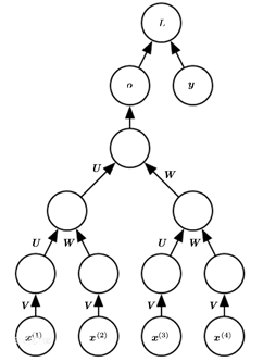
The CNN can extract features of multiple levels and scales, thanks to its unique structure. In this paper, a multilayer RNN (Figure 1) is introduced to improve the CNN structure for deep feature extraction from varied input images. The multilayer RNN can reduce the dimension of each feature by using the same weight set on each layer and selecting suitable receptive fields.
Figure 1. Structure of the RNN
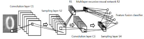
In the improved CNN (Figure 2), the shallow features of the input image are extracted by the first convolutional layer, while the deep features are learned by the second convolutional layer and the multilayer RNN; both shallow and deep features are fused and then inputted to the classifier.
As shown in Figure 2, the first RNN (R1) is connected to the sampling layer S2 of the CNN. The m×m feature map from S2 is inputted into the R1, which has k layers. The receptive fields of the first RNN are 1×1 in size, without any overlap between them. After passing through R1, the feature map becomes m/l×m/l in size, and serves as the input of the multilayer RNN (R2). In R2, the m/l×m/l feature map is reduced to m/l2× m/l2 in size through the first layer; the dimension reduction goes on layer by layer, until the feature map becomes 1×1 in size.
Figure 2. Structure of the improved CNN
The CNN structure was further improved by optimizing key parameters like activation function, learning rate and the number of kernels.
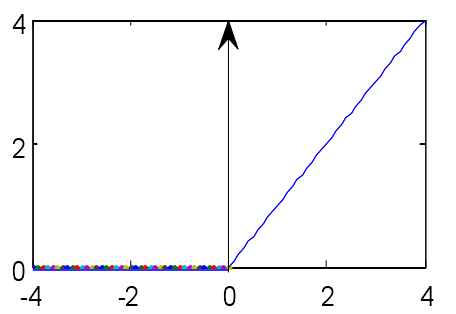
In terms of activation function, the commonly used sigmoid function was replaced with the ReLU, because the latter is suitable for sparse activation of neurons, and capable of getting the activation value with only a threshold. As shown in Figure 3, if x<0, the output of ReLU is always zero; if x>0, the ReLU output increases with x value.
Figure 3. The curve of ReLU
Three activation functions, sigmoid, tanh and ReLU, were separately taken as the activation function of the improved CNN, and tested on the ImageNet dataset [17], the most popular dataset in image recognition. The experimental results (Table 1) show that ReLU outperformed the other two functions in recognition accuracy.
Table 1. Experimental results of the three activation functions
|
Activation function |
Sigmoid |
Tanh |
ReLU |
|
False acceptance rate (FAR) (%) |
1.75 |
1.63 |
1.31 |
Since the ReLU value increases continuously, the learning rate must be set appropriately to control the convergence speed in a suitable range.
The adaptive learning rate algorithm can verify whether the network error is reduced through parameter adjustment, and ensure that the network is trained at the maximum learning rate. Therefore, this algorithm was employed to update the learning rate with the training of the improved CNN, speeding up the convergence. The adaptive learning rate can be adjusted by:
$\delta(\mathrm{n}+1)=\left\{\begin{array}{ll}1.05 \delta(\mathrm{n}) & \mathrm{E}(\mathrm{n})<\mathrm{E}(\mathrm{n}-1) \\ 0.75 \delta(\mathrm{n}) & \mathrm{E}(\mathrm{n})>1.05 \mathrm{E}(\mathrm{n}-1) \\ \delta(\mathrm{n}) & \text { otherwise }\end{array}\right.$
The recognition accuracy and computing complexity of the improved CNN are also affected by the number of kernels. In the convolutional layer, each kernel is responsible for extracting a feature from the input image, i.e. the number of kernels equals that of learned features.
To identify the optimal number of kernels, ten kernel combinations were designed and tested on the ImageNet dataset. As shown in Table 2, the improved CNN did not achieve a high accuracy, when there were only a few kernels. With the growing number of kernels, more and more new features were extracted, and the FAR of the network started to decline. However, the decline of the FAR was no longer prominent, as the number of kernels increased from 9 to 10. Further increase in the number of kernels only extended the training time, without enhancing the recognition performance.
Table 2. Experimental results of different kernel combinations
|
(C1, C3) |
FAR (%) |
|
(1, 2) |
8.41 |
|
(2, 3) |
5.53 |
|
(3, 5) |
3.49 |
|
(4, 6) |
2.77 |
|
(5, 10) |
1.87 |
|
(6, 12) |
1.76 |
|
(7, 14) |
1.73 |
|
(8, 16) |
1.70 |
|
(9, 17) |
1.68 |
|
(10, 20) |
1.68 |
3.2 Improved CNN training algorithm
In the traditional CNN, the cost function is generally the mean square error function. This function needs lots of tagged samples and consumes a long time to train the network. To solve the problems, this paper proposes an improved CNN training algorithm.
Once the CNN parameters were trained, the Fisher criterion was introduced to the error function of the network. The Fisher criterion is a classical criterion function in linear discriminant analysis, which aims to optimize the projection direction and classification effect. Under this criterion, the weights are updated iteratively and the network parameters are adjusted, thereby minimizing the residual error between actual and expected outputs and reducing the distance between samples of the same category.
To improve the classification effect, this paper improves the global mean and reduces the proportion of outliers in all samples, using the weighted Fisher criterion. Let S={s1, s2,…, sN} be a set of original images, with si being the subset of images of category i, and sij be the j-th sample in category i. Then, the similarity SB between images in different categories and that SW between images within the same category can be respectively defined as:
$S_{B}=\sum_{i=1}^{C} q_{i}\left(a_{i}-a\right)\left(a_{i}-a\right)^{T}$
$S_{W}=\sum_{i=1}^{C} q_{i} \sum_{j=1}^{n_{i}}\left(s_{i j}-a_{i}\right)\left(s_{i j}-a_{i}\right)^{T}$
where, ai is the mean of i-th category samples; a is the mean of all samples; qi is the priori probability of i-th category samples; qi is the number of samples in the i-th category. Then, the Fisher criterion can be defined as:
$\mathrm{F}(\mathrm{W})=\frac{\left|\mathrm{W}^{\mathrm{T}} \mathrm{S}_{\mathrm{B}} \mathrm{W}\right|}{\left|\mathrm{W}^{\mathrm{T}} \mathrm{S}_{\mathrm{W}} \mathrm{W}\right|}$
Next, the weighted Fisher criterion was proposed to enhance the classification ability of linear discriminant algorithm and reduce the leading role of edge category. The similarity between images in different categories, a.k.a. the inter-category similarity, can also be expressed as:
$S_{B}=\sum_{i=1}^{C-1} \sum_{j=i+1}^{C} q_{i} q_{j}\left(a_{i}-a_{j}\right)\left(a_{i}-a_{j}\right)^{T}$
Then, the function of weighted inter-category similarity was constructed to assign different weights to the means of samples in different categories. This function can be written as a weighted inter-category scatter matrix:
$S_{B}^{W}=\sum_{i=1}^{C-1} \sum_{j=i+1}^{C} \sigma\left(d_{i j}\right) q_{i} q_{j}\left(a_{i}-a_{j}\right)\left(a_{i}-a_{j}\right)^{T}$
where, dij=(ai-aj)T(ai-aj) is the distance between the mean of the i-th category samples and that of the j-th category samples; s(dij)is the weight function whose value is negatively correlated with dij:
$\sigma(\mathrm{x})=\frac{1}{2 \mathrm{x}^{2}} \mathrm{f}\left(\frac{\mathrm{x}}{2 \sqrt{2}}\right)$
$f(x)=\frac{2}{\sqrt{x}} \int_{0}^{x} e^{-t^{2}} d t$
Substituting $S_{\mathrm{B}}^{\mathrm{W}}$ for SB in Fisher criterion, the weighted Fisher criterion function can be obtained as:
$\mathrm{F}^{\mathrm{W}}(\mathrm{W})=\frac{\left|\mathrm{W}^{\mathrm{T}} \mathrm{S}_{\mathrm{B}}^{\mathrm{W}} \mathrm{W}\right|}{\left|\mathrm{W}^{\mathrm{T}} \mathrm{S}_{\mathrm{W}} \mathrm{W}\right|}$
The weighted Fisher criterion was further improved to reduce the proportion of outliers in the means of all categories. The distances between i-th category samples can be added up as:
$\mathrm{D}_{\mathrm{i}}=\sum_{\mathrm{j}=1, \mathrm{j} \neq \mathrm{i}}^{\mathrm{C}} \mathrm{d}_{\mathrm{ij}}$
where, Qi is the ratio of the distance between i-th category samples to the minimum distance between these samples:
$\mathrm{Q}_{\mathrm{i}}=\frac{\mathrm{D}_{\mathrm{i}}}{\mathrm{D}_{\mathrm{min}}}$
where, Dmin=min{D1, D2,…, Dc}. The improved means of all categories can be calculated as:
$\mathrm{a}^{*}=\frac{1}{\mathrm{C}} \sum_{\mathrm{i}=1}^{\mathrm{C}} \sigma_{\mathrm{a}}\left(\mathrm{Q}_{\mathrm{i}}\right) \mathrm{a}_{\mathrm{i}}$
$\sigma_{\mathrm{a}}(\mathrm{x})=\frac{1}{\mathrm{x}}$
The new method to calculate the inter-category dispersion can be defined as:
$S_{\mathrm{B}}^{*}=\sum_{i=1}^{C} \sigma_{\mathrm{b}}\left(Q_{\mathrm{i}}\right) q_{\mathrm{i}} \mathrm{q}_{\mathrm{j}}\left(\mathrm{a}_{\mathrm{i}}-\mathrm{a}^{*}\right)\left(\mathrm{a}_{\mathrm{i}}-\mathrm{a}^{*}\right)^{\mathrm{T}}$
$\sigma_{\mathrm{b}}(\mathrm{x})=\sigma(\mathrm{x})$
Therefore, the improved weighted Fisher criterion can be defined as:
$\mathrm{F}^{*}(\mathrm{W})==\frac{\left|\mathrm{W}^{\mathrm{T}} \mathrm{S}_{\mathrm{B}}^{*} \mathrm{W}\right|}{\left|\mathrm{W}^{\mathrm{T}} \mathrm{S}_{\mathrm{W}} \mathrm{W}\right|}$
In the traditional CNN, the network loss is usually measured by the least square error function. Here, the improved weighted Fisher criterion is introduced to optimize the traditional loss function of the CNN, creating a CNN algorithm based on the improved weighted Fisher criterion.
The mean $A^{(i)}$ of i-th category samples can be calculated as:
$A^{(i)}=\frac{1}{n} \sum_{j=1}^{n} l_{W, b}\left(x^{i j}\right)$
The mean of the samples from all categories can be calculated by:
$A^{\prime(i)}=\frac{1}{n} \sum_{i=1}^{n} \sigma_{a}\left(Q_{i}\right) A^{(i)}$
The inter-category similarity MB, i.e. the sum of distances of all category means, and the intra-category similarity MW, i.e. the sum of distances between all samples and their category means, can be respectively calculated by:
$\mathrm{M}_{\mathrm{B}}=\frac{1}{2} \sum_{\mathrm{i}=1}^{\mathrm{m}} \sum_{\mathrm{j}=\mathrm{i}+1}^{\mathrm{m}}\left\|\sigma\left(\mathrm{Q}_{\mathrm{i}}\right)\left(\mathrm{A}^{\prime(\mathrm{i})}-\mathrm{A}^{\prime(\mathrm{j})}\right)\right\|^{2}$
$\left.\mathrm{M}_{\mathrm{W}}=\frac{1}{2} \sum_{\mathrm{i}=1}^{\mathrm{m}} \sum_{\mathrm{j}=1}^{\mathrm{n}} \| \mathrm{l}_{\mathrm{W}, \mathrm{b}}\left(\mathrm{x}^{\mathrm{ij}}\right)-\mathrm{A}^{(\mathrm{i})}\right) \|^{2}$
Then, the loss of the improved CNN can be described as:
$\mathrm{M}=\mathrm{M}(\mathrm{W}, \mathrm{b})-\vartheta \mathrm{M}_{\mathrm{B}}+\mu \mathrm{M}_{\mathrm{W}}$
where, $\vartheta$ and m are the adjustment coefficients between 0 and 1; M(W, b) is least square error cost function.
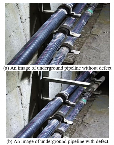
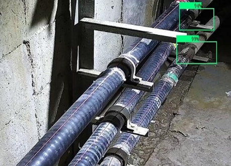
To verify its performance, the improved CNN was compared with LeNet-5 and backpropagation neural network (BPNN) through an experiment on 7,200 samples from the underground pipeline image. The samples were divided into a training set of 6,000 images and a test set of 1,200 images. Figures 4 and 5 are two samples used for our experiment.
Figure 4. Images of underground pipelines
As shown in Table 3, the improved CNN achieved a higher recognition rate than the two contrastive networks. The recognition rate of the improved CNN was 1.17% higher than that of LeNet-5, which is a traditional CNN, thanks to the RNN on the second layer. The results show that the RNN can effectively learn deep features.
Table 3. Comparison of recognition rate
|
Model |
Recognition rate (%) |
|
BPNN |
91.26 |
|
LeNet-5 |
96.58 |
|
Improved CNN |
97.75 |
Figure 5. Recognition result of underground pipeline with defect
Figure 5 shows the improved CNN’s recognition result of Figure 4. It can be seen that our algorithm achieved good recognition effect with fewer training samples and iterations than the other methods. The good effect is attributable to the improved weighted Fisher criterion in our algorithm.
Another experiment was conducted to explore the relationship between the number of iterations and the recognition rate. The results in Table 4 show that the improved CNN had a much higher recognition rate than the traditional CNN, when the number of iterations was small. In this case, our algorithm can realize the same recognition effect in a relatively short time. When the number of iterations was high, the improved CNN was slightly better than the traditional CNN in recognition effect.
Table 4. Relationship between the number of iterations and recognition rate
|
Number of iterations |
5 |
10 |
15 |
20 |
|
Traditional CNN |
85.27% |
88.36% |
92.61% |
95.56% |
|
Improved CNN |
92.23% |
93.21% |
95.37% |
96.87% |
This paper develops an image recognition method for defect detection in urban underground pipelines. The classic CNN was improved with multilayer RNN and improved weighted Fisher criterion, and verified through contrastive experiments on images of underground pipelines. The experimental results show that the improved CNN achieved good recognition rate with a few iterations and training samples. The proposed algorithm can extract diverse features from underground pipeline images.
[1] Li, W., Ling, W., Liu, S., Zhao, J., Liu, R., Chen, Q., Qiang, Z., Qu, J. (2011). Development of systems for detection, early warning, and control of pipeline leakage in drinking water distribution: A case study. Journal of Environmental Sciences, 23(11): 1816-1822. https://doi.org/10.1016/s1001-0742(10)60577-3
[2] Duan, H.F. (2015). Uncertainty analysis of transient flow modeling and transient-based leak detection in elastic water pipeline systems. Water Resources Management, 29(14): 5413-5427. https://doi.org/10.1007/s11269-015-1126-4
[3] Yang, J., Zhang, X. (2012). Feature-level fusion of fingerprint and finger-vein for personal identification. Pattern Recognition Letters, 33(5): 623-628. https://doi.org/10.1016/j.patrec.2011.11.002
[4] Fekri-Ershad, S. (2019). Gender classification in human face images for smart phone applications based on local texture information and evaluated Kullback-Leibler divergence. Traitement du Signal, 36(6): 507-514. https://doi.org/10.18280/ts.360605
[5] Zhang, X.L., Liu, F., Ne, Y. (2014). Rapid detection of nitrogen content and distribution in oilseed rape leaves based on hyperspectral imaging. Spectroscopy and Spectral Analysis, 34(9): 2513-2518. https://doi.org/10.3964/j.issn.1000-0593(2014)09-2513-06
[6] Meng, W.L., Mao, C.Z., Zhang, J., Wen, J., Wu, D.H. (2019). A fast recognition algorithm of online social network images based on deep learning. Traitement du Signal, 36(6): 575-580. https://doi.org/10.18280/ts.360613
[7] Sinha, S.K., Karray, F. (2002). Classification of underground pipe scanned images using feature extraction and neuro-fuzzy algorithm. IEEE Transactions on Neural Networks, 13(2): 393-401. https://doi.org/10.1109/72.991425
[8] Wang, X., Peter, W.T., Mechefske, C.K., Hua, M. (2010). Experimental investigation of reflection in guided wave-based inspection for the characterization of pipeline defects. NDT & E International, 43(4): 365-374. https://doi.org/10.1016/j.ndteint.2010.01.002
[9] Lu, N., Mabu, S., Wang, T., Hirasawa, K. (2013). An efficient class association rule-pruning method for unified intrusion detection system using genetic algorithm. IEEJ Transactions on Electrical and Electronic Engineering, 8(2): 164-172. https://doi.org/10.1002/tee.21836
[10] He, J., Zou, Y., Ma, Y., Chen, G. (2011). Assistant design system of urban underground pipeline based on 3D virtual city. Procedia Environmental Sciences, 11(2011): 1352-1358. https://doi.org/10.1016/j.proenv.2011.12.203
[11] Feng, S., Liu, D., Cheng, X., Fang, H., Li, C. (2017). A new segmentation strategy for processing magnetic anomaly detection data of shallow depth ferromagnetic pipeline. Journal of Applied Geophysics, 139: 65-72. https://doi.org/10.1016/j.jappgeo.2017.02.009
[12] Jia, Z., Hao, Y., Xie, H. (2006). The degradation assessment of epoxy/mica insulation under multi-stresses aging. IEEE Transactions on Dielectrics and Electrical Insulation, 13(2): 415-422. https://doi.org/10.1109/TDEI.2006.1624287
[13] Heiberg, T., Kriener, B., Tetzlaff, T., Casti, A., Einevoll, G.T., Plesser, H.E. (2013). Firing-rate models capture essential response dynamics of LGN relay cells. Journal of Computational Neuroscience, 35(3): 359-375. https://doi.org/10.1007/s10827-013-0456-6
[14] Looe, H.K., Delfs, B., Poppinga, D., Harder, D., Poppe, B. (2018). 2D convolution kernels of ionization chambers used for photon-beam dosimetry in magnetic fields: the advantage of small over large chamber dimensions. Physics in Medicine & Biology, 63(7): 075013. https://doi.org/10.1088/1361-6560/aab50c
[15] Lee, H., Kwon, H. (2017). Going deeper with contextual CNN for hyperspectral image classification. IEEE Transactions on Image Processing, 26(10): 4843-4855. https://doi.org/10.1109/TIP.2017.2725580
[16] Dong, Y., Zhang, H., Wang, C., Wang, Y. (2019). Fine-grained ship classification based on deep residual learning for high-resolution SAR images. Remote Sensing Letters, 10(11): 1095-1104. https://doi.org/10.1080/2150704X.2019.1650982
[17] Russakovsky, O., Deng, J., Su, H., Krause, J., Satheesh, S., Ma, S., Berg, A.C. (2015). Imagenet large scale visual recognition challenge. International Journal of Computer Vision, 115(3): 211-252. https://doi.org/10.1007/s11263-015-0816-y