Xiao Tang* | Ting Zeng | Benxiang Ding | Yang Tan
© 2020 IIETA. This article is published by IIETA and is licensed under the CC BY 4.0 license (http://creativecommons.org/licenses/by/4.0/).
OPEN ACCESS
The key of salient object detection is to extract the most attractive area in the scene. This paper fully explores the hierarchical cognitive mechanism of visual information, combines color contrast and depth contrast, and puts forward a salient object detection algorithm for the RGB-D image. Three saliency maps were prepared, namely, initial saliency map, middle saliency map and advanced saliency map. The three maps were then fused into a final saliency map. The proposed method was compared with six popular salient object detection methods on three RGB-D image datasets. The comparison shows that our algorithm achieved the best results in accuracy, recall rate and F-value. The research findings shed important new light on salient object detection in RGB-D images.
cognitive mechanism, salient object detection, RGB-D image, saliency map
The human eyes have a limited ability to process the information from the complex scene of the surroundings. Guided by the visual attention mechanism (VAM), our eyes will automatically focus on the objects of interest in a scene, rather than deal with every part of a scene. These objects are extracted accurately and quickly from the complex scene through data filtering by the VAM.
The computer offers a convenient tool to capture the key information in the scene [1]. As a result, the VAM has been repeatedly simulated by computer to realize efficient processing of the scene information. In recent years, many have explored salient object detection in the field of computer vision, and applied this technique in such fields as data transmission, image scaling, image segmentation and object recognition [2-5].
The existing detection models for salient objects are either driven by data or driven by tasks. The data-driven model looks for salient objects in the scene from the bottom up, while the task-driven model identifies salient objects from the top down based on prior knowledge. There are more data-driven models than task-driven ones.
The data-driven models focus on two problems: fixed point prediction [6] and salient region detection [7]. Both problems are highly ill-posed with little supervision information. Therefore, some hypotheses must be provided for salient object detection. Based on the type of hypotheses, the salient object detection models can be divided into cognitive models, heuristic models and learning models.
Drawing on the hierarchical cognitive mechanism of visual information, this paper develops a novel algorithm for salient object detection in the RGB-D image. First, a primary saliency map was obtained based on color contrast and depth contrast. Next, the middle saliency map was calculated through multi-scale segmentation and graph cut smoothing. After that, the advanced saliency map was plotted by semi-supervised extreme learning machine (ELM). On this basis, the three maps were combined into the final saliency map. Finally, the proposed algorithm was compared with several popular methods for salient object detection in images.
The cognitive models for salient object detection mimic the VAM of humans. Drawing on the VAM, Le Meur et al. [8] designed a data-driven model for salient object detection, which makes full use of features like contrast sensitivity function, perceptual decomposition, visual mask, and center-surrounding difference. Sun and Bin [9] simulated the complex network of neurons in the visual cortex as a graph, in which each node is a neuron and the nodes communicate through feature difference and spatial distance, and then created a Markov chain to model the data processing of the VAM. Yang et al. [10] held that the saliency of an object depends on its sparsity in the scene, and considered the salient regions as the focus of visual search, eliminating the need to process lots of redundant information in the natural scene.
The heuristic models for salient object detection are the latest results of active vision. Based on visual contrast, Karczmarek et al. [11] designed a fuzzy saliency growth method to detect the salient part of the scene. Mandeel et al. [12] developed a global and spatial region contrast algorithm to extract the region of interest (ROI), and obtained a full resolution saliency map through histogram-based method, which computes the Euclidean distance between color histograms of image blocks. Chen and Chu [13] proposed the spectral residual method to extract the salient part of the image: the redundant part was approximated by the local average filter and the logarithmic spectral filter, and removed from the input image. Inspired by quaternion Fourier transform, Wang and Wang [14] proposed a salient object detection method and applied it to process video sequences. Wan et al. [15] confirmed that the image foreground is sparse in the spatial domain, and put forward a novel theory on image representation, which can be used to approximate the foreground position in the image.
The learning models for salient object detection rely on conditional random fields to learn various image features, namely, multi-scale contrast, center-surrounding histogram, and color spatial distribution. Qian et al. [16] used conditional random fields to learn novel image descriptors, and then judges whether an object is salient in the scene. Through random forest regression, Jog et al. [17] initialized the saliency map, redefined the saliency value through high-dimensional color transform, and detected the salient part of the image. Liu et al. [18] designed a 2D Gaussian filter to highlight the position near the image center, and thus improved the results of salient object detection. Guo et al. [19] found that the boundary effect distorts the area under curve (AUC) and other saliency evaluation indices, and suggested eliminating the boundary effect before salient object detection. Based on the absorption Markov chain, Zhang et al. [20] created a novel learning model for salient object detection: the node saliency was defined as the absorption time from each node to the absorption node; the background was defined as the boundary super-pixel. Lu et al. [21] proposed a salient object detection method based on error reconstruction: the background super-pixel was regarded as the base for sparse and dense representations, and the reconstruction error was used to describe the saliency of image parts.
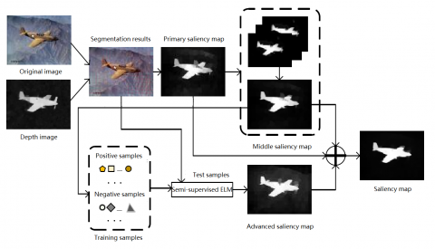
According to the hierarchical cognitive mechanism of visual information, this paper puts forward a novel algorithm for salient object detection in the image, in which the original image is segmented based on the depth information. The block diagram of the proposed algorithm is illustrated in Figure 1.
Figure 1. The block diagram of the proposed algorithm
As shown in Figure 1, the RGB-D image was subjected to super-pixel segmentation based on depth information. Then, three saliency maps were acquired: the primary saliency map, the middle saliency map and the advanced saliency map. The primary saliency map was obtained based on visual contrast; the middle saliency map was calculated through multi-scale segmentation and graph cut smoothing; the advanced saliency map was plotted by semi-supervised ELM. Finally, the three maps were combined into the final saliency map.
3.1 Primary saliency map
The early methods for salient object detection mainly deal with single pixels or regular image units, but the detection results are generally unsatisfactory. This gives rise to the salient object detection methods based on irregular image units [22]. The new methods enjoy excellent detection results and generate high-quality saliency maps.
Color and depth are important external information that can be acquired by the human VAM. Hence, the RGB-D data must be considered in computer simulation of the VAM. Visual contrast, the brightness/color difference that makes an object distinguishable, is critical to the calculation of low visual saliency.
For a given set of RGB-D images, each image was segmented into super-pixels to preserve the internal structure and improve computing efficiency. To prevent over-segmentation, the traditional sequence-and ligation-independent cloning (SLIC) method was improved with depth information. The improved SLIC method consists of the following steps:
Step 1. Segment the original image into super-pixels by the SLIC method.
Step 2. Normalize the depth data of the image and map the normalized result to [0, 255]. Then, calculate the average depth of each super-pixel area, which was identified in Step 1, at the corresponding position of the depth image.
Step 3. If the depth difference between two adjacent areas is smaller than 10, merge the two areas and recalculate the number of areas.
Step 4. Describe each area with the average position of each super-pixel, and the average values of color and depth features: $x=\{R, G, B, L, A, B, d, x, y\}$. Then, the entire input image can be expressed as $X=\left\{x_{1}, x_{2} \ldots \ldots x_{N},\right\} \in \mathbb{R}^{M \times N}$, where M is the feature dimension, and N is the total number of super-pixels.
The boundary area is often regarded as the background of the image. Because the boundary area tends to contain noises, the low-rank decomposition of the boundary template was performed to de-noise this area. Considering the difference of super-pixels in the feature space, the contrast of a super-pixel relative to the pure boundary area can be defined as:
$S_{1}(i)=\left(\sum_{j=1}^{P} \frac{n_{i}}{N} * d\left(x_{i}, x_{j}\right)\right) \times q(x . y)$ (1)
where, P represents the total number of super-pixels in the pure boundary area; ni is the total number of pixels in the i-th super-pixel area; N is the total number of pixels in the entire image; d(xi,xj)is the Euclidean distance in the feature space between super-pixels i and j in the pure boundary area; g(x.y) is a measure of the distance between the center (x.y) of super-pixel i and the image center $\left(x_{0}, x_{0}\right)$:
$q(x . y)=\exp \left(-\left(x-x_{0}\right)^{2} /\left(2 \beta_{x}^{2}\right)\right.$
$\left.-\left(y-y_{0}\right)^{2} /\left(2 \beta_{y}^{2}\right)\right)$ (2)
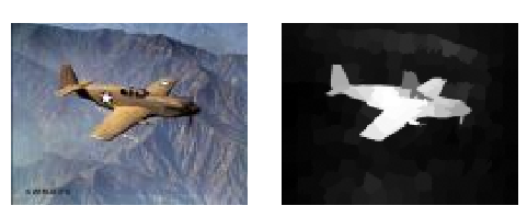
where, bx and by are 1/3 of the length and width of the image, respectively. Therefore, the closer a super-pixel is to the image center, the greater its saliency value. By formula (1), the saliency values of all super-pixels were obtained. Then, the values were assigned to the pixels in the corresponding super-pixel areas, creating the primary saliency map (Figure 2).
Figure 2. An example of primary saliency map
As shown in Figure 2, the pure boundary area basically highlights the salient part of the image, thanks to the selection and de-nosing of this area, and the object position could be roughly identified. Nevertheless, the background noises around the salient object should be further suppressed by processing the primary saliency map based on the contrast of the pure boundary area.
3.2 Middle saliency map
Most salient object detection methods smooth the saliency map through Gaussian filtering. On the upside, the salient object can be detected more accuracy after the filtering. On the downside, the saliency map becomes fuzzier, adding to the difficulty of detection. This paper further smooths the primary saliency map I0 by graph-cut. Based on the contrast of the pure boundary area, a binary map was developed to represent the foreground and background areas of the primary saliency map.
Firstly, the original image was abstracted as an undirected graph G=(V, E, W), where V is the set of super-pixel nodes, E is the set of undirected edges between super-pixel nodes, and W is a set of weights of the undirected edges (connection weights) between each super-pixel node, foreground terminal node and virtual background node. Then, the connection weight between each super-pixel node and the foreground terminal node is a salient value of the saliency map I0.
For each pixel $p,$ the set $W$ can be split into two parts: $\left\{W^{a}(p)\right\}$ and $\left\{W^{b}(p)\right\} .$ Then, the connection weight $T^{a}(p)$ between super-pixel $p$ and the foreground terminal node, and that $T^{b}(p)$ between super-pixel $p$ and the virtual background node can be respectively expressed as:
$T^{a}(p)=I_{0}(p), T^{b}(p)=1-M_{0}(p)$ (3)
In general, the foreground mask M1 is created through minimum cost reduction. Here, the maximum flow algorithm [23] is introduced to measure the probability that each node belongs to the foreground, and M1 is defined as a binary map containing only foreground and background information. Sometimes, errors might occur in the differentiation between foreground and background. Hence, the primary saliency map M0 and the binary map M1 must be considered simultaneously. Then, the saliency map processed by graph-cut can be defined as:
$S=\frac{M_{0}+M_{1}}{2}$ (4)
The salient object detection is greatly affected by the segmentation scale. If the segmentation is conducted on a single scale, the saliency maps are often not analyzed in a comprehensive manner, and the detection algorithms are sensitive to the number of super-pixels. After all, the salient objects in real-world scenes or images are not of the same size. To preserve the structural information, it is critical to analyze the saliency maps at multiple scales.
In this paper, the original image is segmented at multiple scales to promote salient object detection. Specifically, the RGB-D image was divided at four different scales (L=4), the saliency map was calculated at each scale separately, and the four maps were fused into one comprehensive map. Each saliency map was calculated by:
$S_{2}(I)=\sum_{l=1}^{L} S\left(I^{l}\right)$ (5)
where, $I^{l}$ is the different scales. The final results were normalized to output the detection results of multi-scale salient objects.
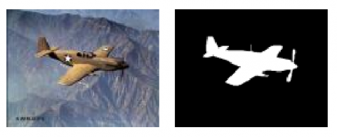
As shown in Figure 3 below, the middle saliency map was closer to the standard map, for the multi-scale fusion solves the imbalance of detection results on the single scale, and alleviates false detection and missed detection.
Figure 3. An example of middle saliency map
3.3 Advanced saliency map
The advanced saliency map was mainly prepared with the semi-supervised ELM [24]. The ELM, a feedforward neural network with a single hidden layer, randomly generates the input weight and hidden layer bias, and analyzes the output weight. In this way, the technique overcomes the defects of gradient-based training algorithms, namely, as local optimization, inefficient learning and slow learning.
The semi-supervised learning of the ELM is based on two assumptions:
(1) All labeled samples $X_{s}$ and unlabeled samples $X_{u}$ obey the same marginal distribution $p_{x}$
(2) Two close points $x_{a}$ and $x_{b}$ should have similar conditions probabilities $p\left(y | x_{a}\right)$ and $p\left(y | x_{b}\right)$
Under the above assumptions, the loss minimization function can be expressed as:
$L_{m}=\frac{1}{2} \sum_{a, b} w_{a b}\left\|P\left(y / x_{a}\right)-P\left(y | x_{b}\right)\right\|^{2}$ (6)
where, $w_{i j}$ is the similarity between the sample $x_{a}$ and $x_{b}$ $\boldsymbol{W}=\left[w_{a b}\right]$ is a sparse similarity matrix. The similarity can be computed by the Gaussian function $\exp \left(-|| x_{a}-x_{b}||^{2} / 2 \sigma^{2}\right)$ The similarity value falls within (0,1)
The conditional probability can be approximated as:
$\hat{L}_{m}=\frac{1}{2} \sum_{a, b} w_{a b}\left\|\hat{y}_{a}-\hat{y}_{b}\right\|^{2}$ (7)
where, $\hat{y}_{a}$ and $\hat{y}_{b}$ are the prediction categories of sample $\mathbf{x}_{a}$ and $x_{b},$ respectively. The conditional probability can be written as a matrix:
$\hat{L}_{m}=\operatorname{Tr}\left(\hat{Y}^{T} \boldsymbol{L} \hat{\boldsymbol{Y}}\right)$ (8)
where, $\operatorname{Tr}(\cdot)$ is the trace of matrix; $\boldsymbol{L}=\boldsymbol{D}-\boldsymbol{W}$ is the obtained Laplacian matrix; $\boldsymbol{D}$ is the diagonal matrix:
$D_{a a}=\sum_{b=1}^{1+N} w_{a, b}$ (9)
For semi-supervised learning, the labeled samples in the training set are denoted as $\left\{\boldsymbol{X}_{s}, \boldsymbol{Y}_{s}\right\}=\left\{x_{i}, y_{i}\right\}_{i=1}^{s},$ and the unlabeled samples in that set as $X_{u}=\left\{x_{i}\right\}_{i=1}^{u},$ where $s$ and $u$ are the total number of all labeled and unlabeled samples, respectively.
If there are a few labelled samples, the semi-supervised ELM will balance the regularization parameters with unlabeled data, thus improving the classification accuracy. The loss function can be expressed as:
$\min _{\delta \in \mathbb{R}^{n_{h} \times n_{0}}} \frac{1}{2}\|\delta\|^{2}+\frac{1}{2} \sum_{i=1}^{s} c_{i}\left\|e_{i}\right\|^{2}+\frac{\lambda}{2} \operatorname{Tr}\left(F^{\tau} S F\right)$ (10)
s.t.
$h\left(x_{i}\right)=y_{i}^{T}-e_{i}^{T}, i=1, \dots, s$
$f_{i}=h\left(x_{i}\right) \delta, i=1, \ldots, l+u$
where, $n_{h}$ is the number of hidden layer neurons; $n_{0}$ is the output dimension; $\delta \epsilon \mathbb{R}^{n_{h} \times n_{0}}$ is the output weight connecting the hidden layer and the output layer; $c_{i}=c_{0} / N_{t_{i}}$ is the penalty coefficient of the training error; $c_{0}$ is a default parameter of traditional ELM; $N_{t_{i}}$ is the total number of samples in the $t_{i}$ -th category; $S \epsilon \mathbb{R}^{(s+u) \times(s+u)}$ is a Laplacian matrix of labeled data and unlabeled data; $F \epsilon \mathbb{R}^{(s+u) \times n_{0}}$ is the output matrix whose $i$ -th row equals the ELM output $f\left(x_{i}\right) ; \lambda$ is the adjusting parameter; $\mathrm{h}\left(x_{i}\right) \in \mathbb{R}^{s \times n_{h}}$ is the output vector corresponding to the hidden layer of sample $x_{i} ; e_{i} \in \mathbb{R}^{n_{0}}$ is the output error corresponding to the $i$ -th training sample.
The solution of the semi-supervised ELM can be calculated as:
$\beta^{*}=\left(I_{n_{h}}+H^{T} C H+\lambda H^{T} L H\right)^{-1} H^{T} C \tilde{Y}$ (11)
If there are fewer labelled samples than the hidden layer neurons, the solution can be obtained by:
$\beta^{*}=H^{T}\left(I_{n_{h}}+C H H^{T}+\lambda L H H^{T}\right)^{-1} C \tilde{Y}$ (12)
The reliable training samples in the advanced saliency map were derived from the middle saliency map $S_{2}$ in the following manner. First, two saliency thresholds were set up. Next, the average salient value of all pixels in each area was compared with the two thresholds. The super-pixels with greater saliency than the high threshold was taken as positive samples, and labeled as $1 ;$ the super-pixels with smaller saliency than the low threshold was treated as negative samples, and labeled as-1. Then, every training sample is composed of positive and negative samples, and labeled as $\left\{X_{s}, Y_{s}\right\}=\left\{x_{i}, y_{i}\right\}_{i=1}^{s},$ where $s$ is the number of training samples, $x_{i}$ is the eigenvector of the i-th training sample, and $y_{i}=1$ or -1 is the label of the $i$ -th training sample.
Due to the background noise in the middle saliency map, the selected positive and negative samples might contain noises. Hence, the feature matrix of the whole image was selected as test samples for semi-supervised learning, rather than the remaining unlabeled super-pixel samples. Thus, the test sample can be expressed as $X_{u}=\left\{x_{1}, x_{2}, \ldots \ldots x_{n}\right\} \in \mathbb{R}^{M \times N},$ where
$u=N$ is the number of test samples.
The advanced saliency map was derived in the following steps:
Step $1 .$ Input the training samples $\left\{X_{s}, Y_{s}\right\}=\left\{x_{i}, y_{i}\right\}_{i=1}^{s}$ and test samples $X_{u}=\left\{x_{1}, x_{2} \ldots x_{n}\right\} \in \mathbb{R}^{M \times N}$;
Step $2 .$ Construct the Laplacian matrix $S \epsilon \mathbb{R}^{(s+u) \times(s+u)}$ of the map from $\boldsymbol{X}_{s}$ and $\boldsymbol{X}_{u}$;
Step $3 .$ Randomly initialize the input weights and biases of the $n_{h}$ hidden layer neurons of the ELM, calculate the output matrix of the hidden layer neurons $H \in \mathbb{R}^{(s+u) \times n_{h}},$ and select the weight parameters $c_{0}$ and $\lambda$;
Step $4 .$ If $n_{h} \leq N,$ calculate the output weight by formula (11); otherwise, calculate the output weight by formula (12).
Step $5 .$ Construct the mapping function $(x)=h(x) \delta$.
The final result was normalized into (0, 1) as the saliency value of each super-pixel. Through the above steps, the advanced saliency map $S_{3}$ was obtained from the middle saliency map through semi-supervised ELM.
Figure 4. An example of advanced saliency map
As shown in Figure 4, the semi-supervised ELM not only approximates the position of the salient object, but also represents the general shape of the object.
3.4 Fusion of saliency maps
The three saliency maps reflect the hierarchy of our cognitive mechanism. The primary saliency map was calculated using the contrast between each super-pixel and the background. This map facilitates the extraction of local information from the input image, providing more details about the salient object. The middle saliency map was prepared through multi-scale segmentation and graph cut smoothing, which prevents over-segmentation. The advanced saliency map was obtained through semi-supervised ELM, with the global information as the test sample. However, the detection results based on the advanced saliency map are not satisfactory, if the background and foreground are close to each other or the positive and negative samples are highly similar.
Therefore, the three saliency maps were weighted and smoothed by graph cut method, creating a final saliency map:
$s=\gamma_{1} S_{1}+\gamma_{2} S_{2}+\gamma_{3} S_{3}$ (13)
where, $\gamma_{1}, \gamma_{2}$ and $\gamma_{3}$ are balance factors that balance the weights between the three saliency maps. Note that $\gamma_{1}+\gamma_{2}+\gamma_{3}=1$ and $\gamma_{1}<\gamma 2<\gamma_{3},$ i.e. the higher the level, the greater the weight of the map.
To verify its performance, our algorithm was evaluated on three public RGB-D datasets: the NLPR1000 dataset [25], the NJUD400 dataset [26], and the RGBD135 dataset [27]. The NLPR1000 dataset contains 1,000 RGB-D images captured by Microsoft Kinect sensors in indoor and outdoor scenes. The NJUD400 dataset provides 400 high-resolution scene images collected from the Internet, 3D movies, and Fujifilm cameras; the depth map of each image is generated by the optical flow method. The RGBD135 dataset contains 135 indoor scene images with a single target and a complex background; these images are captured by Microsoft Kinect sensors (resolution: 640×480), marked by three observers, and divided into 80 categories.
The experimental parameters were configured as follows: For the middle saliency map, four scales $I^{h}=(h=(1,2,3,4))$ were defined: 100,150,250 and $250 .$ For the advanced saliency map the high threshold was set adaptively at 1.8 times the average of the middle saliency map; the low threshold was fixed at 0.05 For the fusion of the three maps, $\gamma_{1}+\gamma_{2}+\gamma_{3}=1$=0.2, $\gamma_{1}=0.2, \gamma_{2}=0.3$ and $\gamma_{3}=0.5$.
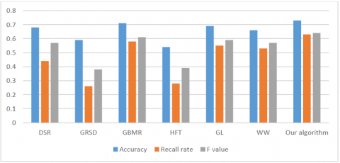
For comparison, our algorithm was compared with six popular salient object detection methods for the image: dynamic stochastic resonance (DSR) method [28], GRSD [29], GBMR [30], HFT [31], GL [32] and WW [33]. None of these algorithms considers the depth information.
Figures 5-7 compare the detection results of our algorithm with those of the six contrastive methods on the NJUD400 dataset, the NLPR1000 dataset and the RGBD135 dataset, respectively. The results of each algorithm were measured by three indices: accuracy, recall rate and F-value.
As shown in Figure 5, our algorithm achieved the highest accuracy, recall rate and F-value. Among the contrastive methods, only the GL method was slightly behind our algorithm in accuracy and recall rate. As shown in Figure 6, our algorithm still boasted the highest F-value, and its recall rate and accuracy were both above the average levels. As shown in Figure 7, our algorithm had obvious advantages over other methods in accuracy, recall rate and F-value.
To sum up, our algorithm has better robustness than the contrastive methods in both single and complex backgrounds. This is attributable to the effective combination of color contrast and depth contrast.
Figure 5. Results comparison on the NJUD400 dataset
Figure 6. Results comparison on the NLPR1000 dataset
Figure 7. Results comparison on the RGBD135 dataset
This paper puts forward a salient object detection algorithm for RGB-D image based on the hierarchical cognitive mechanism of humans. The proposed algorithm mainly covers four steps: preparing the primary saliency map, plotting the middle saliency map, computing the advanced saliency map, and fusing the three maps into a final map. Experimental results show that our algorithm outperformed the popular salient object detection methods in all metrics. With high-quality saliency maps, our algorithm can highlight every salient object in the scene, while alleviating over-segmentation.
The work was supported by Sichuan Science and Technology Program of China (2019YJ0529) and Key Project of Sichuan Education Department of China (18ZA0410).
[1] Intoy, J., Rucci, M. (2020). Finely tuned eye movements enhance visual acuity. Nature Communications, 11(1): 795. https://doi.org/10.1038/s41467-020-14616-2
[2] Liang, Z., Chi, Z., Fu, H., Feng, D. (2012). Salient object detection using content-sensitive hypergraph representation and partitioning. Pattern Recognition, 45(11): 3886-3901. https://doi.org/10.1016/j.patcog.2012.04.017
[3] Cholakkal, H., Johnson, J., Rajan, D. (2018). Backtracking spatial pyramid pooling-based image classifier for weakly supervised top-down salient object detection. IEEE Transactions on Image Processing, 27(12): 6064-6078. https://doi.org/10.1109/TIP.2018.2864891
[4] Tuncer, S.A., Alkan, A. (2019). Spinal cord based kidney segmentation using connected component labeling and K-means clustering algorithm. Traitement du Signal, 36(6): 521-527. https://doi.org/10.18280/ts.360607
[5] Hamdini, R., Diffellah, N., Namane, A. (2019). Robust local descriptor for color object recognition. Traitement du Signal, 36(6): 471-482. https://doi.org/10.18280/ts.360601
[6] Martínez, M.Á., Etchebehere, S., Valero, E.M., Nieves, J.L. (2019). Improving unsupervised saliency detection by migrating from RGB to multispectral images. Color Research and Application, 44(6): 875-885. https://doi.org/10.1002/col.22421
[7] Bavirisetti, D.P., Dhuli, R. (2018). Multi-focus image fusion using multi-scale image decomposition and saliency detection. Ain Shams Engineering Journal, 9(4): 1103-1117. https://doi.org/10.1016/j.asej.2016.06.011
[8] Le Meur, O., Le Callet, P., Barba, D., Thoreau, D. (2006). A coherent computational approach to model bottom-up visual attention. IEEE Transactions on Pattern Analysis & Machine Intelligence, 28(5): 802-817. https://doi.org/10.1109/TPAMI.2006.86
[9] Sun, G.X., Bin, S. (2017). Router-level internet topology evolution model based on multi-subnet composited complex network model. Journal of Internet Technology, 18(6): 1275-1283. https://doi.org/10.6138/JIT.2017.18.6.20140617
[10] Yang, C.T., Chiu, Y.C., Yeh, Y.Y. (2012). Feature saliency affects delayed matching of an attended feature. Journal of Cognitive Psychology, 24(6): 714-726. https://doi.org/10.1080/20445911.2012.683782
[11] Karczmarek, P., Pedrycz, W., Reformat, M., Akhoundi, E. (2014). A study in facial regions saliency: A fuzzy measure approach. Soft Computing, 18(2): 379-391.
[12] Mandeel, T.H., Ahmad, M.I., Isa, M.N.M., Anwar, S.A., Ngadiran, R. (2018). Palmprint region of interest cropping based on Moore-neighbor tracing algorithm. Sensing and Imaging, 19(1): 15-29. https://xs.scihub.ltd/https://doi.org/10.1007/s11220-018-0199-6
[13] Chen, D.Y., Chu, H. (2012). Scale-invariant amplitude spectrum modulation for visual saliency detection. IEEE Transactions on Neural Networks and Learning Systems, 23(8): 1206-1214. https://doi.org/10.1109/TNNLS.2012.2198888
[14] Wang, Q., Wang, Z. (2012). Color image registration based on quaternion Fourier transformation. Optical Engineering, 51(5): 1-9. https://doi.org/10.1117/1.OE.51.5.057002
[15] Wan, M., Gu, G., Qian, W., Ren, K., Chen, Q. (2016). Robust infrared small target detection via non-negativity constraint-based sparse representation. Applied Optics, 55(27): 7604-7612. https://doi.org/10.1364/AO.55.007604
[16] Qian, S., Chen, Z.H., Lin, M.Q., Zhang, C.B. (2015). Saliency detection based on conditional random field and image segmentation. Acta Automatica Sinica, 41(4): 711-724.
[17] Jog, A., Carass, A., Roy, S., Pham, D.L., Prince, J.L. (2017). Random forest regression for magnetic resonance image synthesis. Medical Image Analysis, 35: 475-488. https://doi.org/10.1016/j.media.2016.08.009
[18] Liu, Z., Xue, Y., Yan, H., Zhang, Z. (2011). Efficient saliency detection based on gaussian models. IET Image Processing, 5(2): 122-131. https://doi.org/10.1049/iet-ipr.2009.0382
[19] Guo, S., Lou, S., Liu F. (2016). Multi-ship saliency detection via patch fusion by color clustering. Optics and Precision Engineering, 24(7): 1807-1817.
[20] Zhang, L., Ai, J., Jiang, B., Lu, H.C., Li, X.K. (2018). Saliency detection via absorbing markov chain with learnt transition probability. IEEE Transactions on Image Processing, 27(2): 987-998. https://doi.org/10.1109/TIP.2017.2766787
[21] Lu, H.C., Li, X.H., Zhang, L.H., Ruan, X., Yang, M.H. (2016). Dense and sparse reconstruction error based saliency descriptor. IEEE Transactions on Image Processing, 25(4): 1592-1603. https://doi.org/10.1109/TIP.2016.2524198
[22] Wang, X., Qi, C. (2016). Saliency-based dense trajectories for action recognition using low-rank matrix decomposition. Journal of Visual Communication and Image Representation, 41: 361-374. https://doi.org/10.1016/j.jvcir.2016.10.015
[23] King, V., Rao, S., Tarjan, R. (1994). A faster deterministic maximum flow algorithm. Journal of Algorithms, 17(3): 447-474. https://doi.org/10.1006/jagm.1994.1044
[24] Huang, G.B., Zhu, Q.Y., Siew, C.K. (2006). Extreme learning machine: Theory and applications. Neurocomputing, 70(1-3): 489-501. https://doi.org/10.1016/j.neucom.2005.12.126
[25] Peng, X., Qiao, Y., Peng, Q., Wang, Q.H. (2014). Large margin dimensionality reduction for action similarity labeling. IEEE Signal Processing Letters, 21(8): 1022-1025. https://doi.org/10.1109/LSP.2014.2320530
[26] Zhang, Z., Zhao, M., Chow, T.W.S. (2012). Constrained large Margin Local Projection algorithms and extensions for multimodal dimensionality reduction. Pattern Recognition, 45(12): 4466-4493. https://doi.org/10.1016/j.patcog.2012.05.015
[27] Wan, S., Aggarwal, J.K. (2014). Spontaneous facial expression recognition: A robust metric learning approach. Pattern Recognition, 47(5): 1859-1868. https://doi.org/10.1016/j.patcog.2013.11.025
[28] Zhang, J., Liu, H.J., Wei, Z.H. (2018). Regularized variational dynamic stochastic resonance method for enhancement of dark and low-contrast image. Computers & Mathematics with Applications, 76(4): 774-787. https://doi.org/10.1016/j.camwa.2018.05.018
[29] Chouhan, R., Jha, R.K., Biswas, P.K. (2013). Enhancement of dark and low-contrast images using dynamic stochastic resonance. Image Processing, IET, 7(2): 1-11. https://doi.org/10.1049/iet-ipr.2012.0114
[30] Ju, R., Liu, Y., Ren, T.W., Ge, L., Wu, G.S. (2015). Depth-aware salient object detection using anisotropic center-surround difference. Signal Processing: Image Communication, 38: 115-126. https://doi.org/10.1016/j.image.2015.07.002
[31] Zhang, L., Zhang, Y.N., Yan, H.Q., Gao, Y.F., Wei, W. (2018). Salient object detection in hyperspectral imagery using multi-scale spectral-spatial gradient. Neurocomputing, 291: 215-225. https://doi.org/10.1016/j.neucom.2018.02.070
[32] Tong, N., Lu, H.C., Zhang, Y., Ruan, X. (2015). Salient object detection via global and local cues. Pattern Recognition, 48(10): 3258-3267. https://doi.org/10.1016/j.patcog.2014.12.005
[33] Qu, L.Q., He, S.F., Zhang, J.W., Tian, J.D., Tang, Y.D., Yang, Q.X. (2017). RGBD salient object detection via deep fusion. Image Processing IEEE Transactions on, 26(5): 2274-2285. https://doi.org/10.1109/TIP.2017.2682981