Feng Zhang | Chao Zhang* | Huamin Yang | Lin Zhao
© 2019 IIETA. This article is published by IIETA and is licensed under the CC BY 4.0 license (http://creativecommons.org/licenses/by/4.0/).
OPEN ACCESS
This paper aims to remove the noises of different scales in point cloud data captured by 3D scanners, while preserving the sharp features (e.g. edges) of the model. For this purpose, the authors proposed a point cloud denoising method based on the principal component analysis (PCA) and a self-designed bilateral filter. First, the outliers in the point cloud were divided into isolated outliers and deviation outliers. The former was directly removed, while the latter was moved along the normal vector estimated by the PCA. Next, a bilateral filter was developed based on vertex brightness, vertex position and normal vector. During image processing, the grayscale of the current point was replaced with the weighted mean of the grayscales of its neighborhood points. The weight function is related to the distance and grayscale difference between the current point and neighborhood points. The effectiveness of our method was proved through experiments on actual point clouds. The results demonstrate that our bilateral filter can retain the sharp features of point cloud data, in addition to removing the small-scale noises.
point cloud, 3D scanner, principal component analysis (PCA), bilateral filter
In recent years, it is a research hotspot to reconstruct 3D entities based on multiple 2D images. The emerging 3D sensing technology has made it possible to collect or generate millions of 3D points from the object surface. These data points form a 3D point cloud, providing a discrete representation of continuous surface. The 3D point cloud has been widely applied in robot design, virtual reality (VR) and computer-aided shape design.
However, the 3D point cloud collected by 3D scanners often contain noises, especially on the edge and center [1]. The noises may come from measuring errors or human factors. The noisy data suppress the fineness, and even distort the shape of the reconstructed model. When a 3D entity is modelled based on multi-view images, it is difficult to remove the noises by the reconstruction algorithm, due to its poor ability of fuzzy matching [2, 3]. To smooth the surface of 3D solid model, the point cloud data must be denoised before surface reconstruction.
Noises fall into two categories: high-frequency noises and low-frequency noises. High-frequency noises are outliers in the point cloud. In practice, these outliers are often confused with the high-frequency components of the edges. In this paper, the outliers are further divided into isolated outliers and deviation outliers. The isolated outliers were directly removed, while the deviation outliers were moved along the normal vector estimated by the principal component analysis (PCA).
Next, a bilateral filter was developed based on vertex brightness, vertex position and normal vector. During image processing, the grayscale of the current point was replaced with the weighted mean of the grayscales of its neighborhood points. The weight function is related to the distance and grayscale difference between the current point and neighborhood points. The effectiveness of our method was proved through experiments on actual point clouds.
With the development of 3D sensing technology, the data acquisition mode of 3D scanners has shifted from contact mode to non-contact mode. The contact 3D scanners are still widely used in many fields (e.g. reverse engineering), due to its high precision. Meanwhile, the non-contact 3D scanners, known for its fast scanning speed, has been applied to 3D reconstruction of entities that cannot be measured in contact mode, such as cultural relics and battlefields. Under the effects of hardware and other factors, it is inevitable for the data collected by 3D scanners to contain noises. Thus, the noise suppression of the point cloud is essential to the accuracy of subsequent processing. The model reconstructed from noisy point cloud is often imprecise, calling for preprocessing of the point cloud with a powerful denoising algorithm [4, 5].
Depending on the diffusion modes of noise in all directions, the existing denoising and smoothing algorithms for 3D point cloud can be categorized to anisotropic and isotropic algorithms. The isotropic algorithm is simple, but unable to distinguish between the sharp features (e.g. edges) and noises. Many sharp features will be lost through isotropic denoising. The anisotropic algorithm can retain the sharp features, while removing the noises. However, the good performance comes at a price: high computing load and time complexity. The following are some of the most representative works related to the denoising of point cloud for 3D modelling.
Wu et al. [6] put forward an adaptive Wiener filter (AWF) for 3D meshing based on classification of feature information. Jones et al. [1] developed a non-iterative, feature-preserving mesh smoothing strategy, which predicts the position of each vertex according to the vertex neighborhoods. Cho et al. [2] created a bilateral texture filter that adjusts the vertex positions based on normal line and normal phase. Li et al. [3] applied Laplace operator to the point cloud model, creating a novel algorithm for envelope surface modeling; However, this algorithm may cause over-smoothness and vertex drift. To prevent vertex drift, Xiao et al. [7] calculated the mean curvature of data points on the point cloud model through principal component analysis (PCA), and proposed a denoising method for point cloud model based on mean curvature flow. Collet et al. [8] established a moving minimum quadric surface for the point cloud model, and approximated the noise points to the quadric surface to reduce the noises.
During statistical analysis, the complexity of an entity is positively correlated with the number of variables. Under ideal conditions, more information should be collected with the minimal number of variables. In many cases, most variables of the same entity are correlated with each other. Each variable reflects some information of the entity. Therefore, two correlated variables must have a certain overlap in terms of the entity information embodied in them. The PCA provides an effective tool to remove the redundant closely correlated variables, leaving only a few irrelevant variables. Together, these irrelevant variables can provide the full information of the entity.
Drawing on the existing studies, this paper attempts to further smooth the surface while preserving the sharp features, after denoising the point cloud with the PCA.
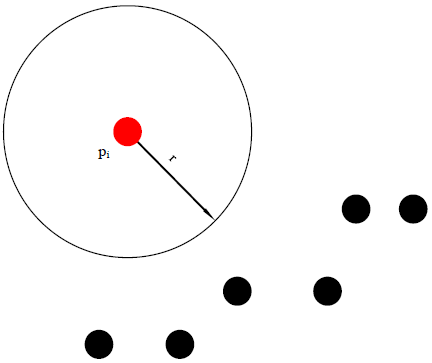
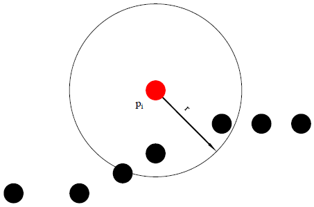
During the collection of point cloud, the 3D scanner is often affected by illumination conditions, the features of surface material and human factors. The obtained point cloud usually contains different degrees of noises [9]. These noises fall into two categories: high-frequency noises and low-frequency noises. High-frequency noises are outliers in the point cloud, and are split here into isolated outliers (as shown in Figure 1) and deviation outliers (as shown in Figure 2).
Let pi be a vertex in the 3D point cloud, and r be the radius of the neighborhood of pi. As shown in Figure 1, if the number of vertices in the neighborhood is smaller than the set threshold N1, then pi is an isolated outlier, and should be moved directly from the point cloud. As shown in Figure 2, a deviation outlier exists on the surface of the object. Direct removal would leave a hole on the surface. Therefore, the PCA was introduced to estimate the normal of the neighborhood of the outlier in the point cloud [10], enabling to outlier to move along the normal vector and avoid vertex drift.
Figure 1. Isolated outliers
Figure 2. Deviation outliers
The normal vector is a fundamental attribute of point cloud. The accuracy of the normal vector directly affects the application effect of point cloud data in reverse engineering, and the rendering and processing of point cloud in many other areas, such as denoising, segmentation, data reduction, and surface reconstruction [11-14]. For surfaces with sharp features, the details of the surfaces are easily lost in point cloud processing, if the normal vector of the feature region, i.e. the transition between surfaces, is not estimated accurately. In this case, it is very difficult to restore the geometric features of the original model on the reconstructed surface.
In recent years, many methods have been developed to estimate the normal vector of point cloud. These estimation methods can be categorized into two groups: local neighborhood fitting, a.k.a. the PCA, and Voronoi/Delaunay method. Chaudhury et al. [15] transform the 3-D problem into 2-D by performing appropriate coordinate transformations to the neighborhood of each 3-D point. Ali et al. [16] review the major tensor decomposition methods with a focus on problems targeted by classical PCA. Namrata et al. [17] studied the dynamic (time-varying) version of the RPCA problem and proposed a series of provably correct, fast, and memory-efficient tracking solutions. The above studies have improved the normal vector estimation of the point cloud to some extent. However, the PCA is a low-pass filtering method that smooths the normal vector at key points [18, 19].
Rente et al. [20] raised the need for efficient point cloud coding solutions in order to offer more immersive visual experiences and better quality of experience to the users. Dey et al. [10] extended the Voronoi poles of a cell in the Voronoi diagram to the large Delaunay sphere, and then estimated the normal vector of point cloud. Vassiliades et al. [21] uses a centroidal Voronoi tessellation (CVT) to divide the feature space into a desired number of regions; it then places every generated individual in its closest region, replacing a less fit one if the region is already occupied. Rakhshanfar et al. [22] propose a method for estimating the image and video noises of different types: white Gaussian (signal-independent), mixed Poissonian-Gaussian (signal-dependent). They assume that the noise variance is a piecewise linear function of intensity in each intensity class. Nevertheless, no Voronoi/Delaunay methods can accurately estimate the normal vector of surfaces with sharp features.
In statistical analysis, the modelling complexity increases with the number of variables of the entity. In many cases, some variables are correlated with each other [23, 24]. The correlation reflects that the variables carry some overlapping information of the entity. Under ideal conditions, the information of the entity should be collected with the minimum number of variables. The PCA offers a desirable tool to reduce the number of variables, because it can delete the variables that are closely correlated, i.e. redundant variables, leaving only pairs of unrelated variables that keep the original information of the entity.
In the light of the above, the PCA was introduced to reduce the dimension of 3D point cloud to a 2D plane, i.e. the tangent plane of the point cloud. Then, the normal vector of the tangent plane pointing towards the camera was taken as the normal vector of the point cloud.
Let p be a point on the tangent plane and pi be a k-nearest neighbor of p. Then, the covariance matrix C of pi can be expressed as:
$C=\left[\begin{array}{l}{p_{i}-p_{1}} \\ {p_{i}-p_{2}} \\ {\cdots} \\ {p_{i}-p_{k}}\end{array}\right]^{T}\left[\begin{array}{c}{p_{i}-p_{1}} \\ {p_{i}-p_{2}} \\ {\cdots} \\ {p_{i}-p_{k}}\end{array}\right]$ (1)
The covariance matrix C can be decomposed into three eigenvectors v1, v2 and v3. The eigenvalues of v1, v2 and v3 are denoted as λ1, λ2 and λ3, respectively. The eigenvector with the smallest eigenvalue is the normal vector of the tangent plane.
The bilateral filter is originally designed for image denoising. In addition to geometric proximity, the bilateral filter also considers the brightness difference between points [25]. Compared with traditional Gaussian filter and mean filter, the bilateral filter can preserve the edge features of the target image [26-28].
For example, Tomasi et al. [25] proposed a noniterative nonlinear bilateral filter to preserve the edge features of images. This filter adopts a domain-weighted process. Unlike the traditional low-pass filter, this filter considers both the distance weight between points and the difference weight between point grayscales. The grayscale L(q) of each point q is described as:
$\widehat{L}(q)=\frac{\sum\limits_{k\in N(q)}{{{W}_{{{\sigma }_{c}}}}(\left\| q-k \right\|)}{{W}_{{{\sigma }_{s}}}}(\left| L(q)-L(k) \right|)L(k)}{\sum\limits_{k\in N(q)}{{{W}_{{{\sigma }_{c}}}}(\left\| q-k \right\|)}{{W}_{{{\sigma }_{s}}}}(\left| L(q)-L(k) \right|)}$ (2)
where, N(q) is the set of points in the neighborhood of q; k is a neighborhood point of q; $(\|q-k\|)$ and $(|L(q)-L(k)|)$ are the geometric distance and brightness distance between q and k, respectively; $W_{\sigma c}$ and $W_{\sigma s}$ are the weighting functions of the distance domain, respectively. To preserve the edge features, the weight coefficient should be small when the grayscale difference is large between two points.
Wang et al. [5] put forward a bilateral filter to denoise the point cloud. However, the filter only takes account of the vertex position and normal vector, failing to utilize the brightness of each vertex.
Therefore, this paper designs a bilateral filter based on vertex brightness, vertex position and normal vector. During image processing, the grayscale of the current point was replaced with the weighted mean of the grayscales of its neighborhood points. The weight function is related to the distance and grayscale difference between the current point and neighborhood points. The denoising of 3D point cloud by the proposed bilateral filter can be described as follows. For the current point p, we have:
$p:=p+\alpha N_{p}$ (3)
where, $\alpha$ is the weight coefficient of the bilateral filter; Np is the normal vector of point p. The value of Np can be solved by the PCA. The point only moves along the normal vector, avoiding the problem of vertex drift. The key of our bilateral filter is to solve the weight coefficient $\alpha$:
$\alpha=\frac{\sum_{k_{i j} \in M\left(p_{i}\right)} W_{\sigma_{c}}(\|q-k\|,|L(q)-L(k)|) W_{\sigma_{s}}\left(\left\langle n_{i}, p_{i}-k_{i j}\right\rangle\right)\left\langle n_{i}, p_{i}-k_{i j}\right\rangle}{\sum_{k \in N(q)} W_{\sigma_{c}}(\|q-k\|,|L(q)-L(k)|) W_{\sigma_{s}}\left(\left\langle n_{i}, p_{i}-k_{i j}\right\rangle\right)}$ (4)
where, $M\left(p_{i}\right)=\left\{p_{i j}\right\} 1 \leq j \leq k$ is a neighborhood point of point pi. In our bilateral filter, the point cloud smoothing is completed through standard 2D Gaussian filtering:
$W_{\sigma}(x, y)=e^{-\frac{x^{2}+y^{2}}{2 \sigma_{c}^{2}}}$ (5)
The weight function for edge feature preservation is realized through 1D Gaussian filtering:
$W_{\sigma}(z)=e^{-\frac{z^{2}}{2 \sigma_{s}^{2}}}$ (6)
where, σc is the standard deviation of brightness and neighborhood distance of vertex pi; σs is the influence factor of the projection of the distance vector from vertex pi to a neighborhood point on the normal vector ni of vertex pi.
The workflow of our bilateral filter can be summed as Algorithm 1 below:
|
Algorithm 1: Bilateral filter (pi, m, σc and σs) |
|
Input: One-point pi K ← a neighborhood point of pi Compute the unit normal vector to the regression plane np from Nm(p) 1. $k_{i j} \in K \mathrm{do}$ 2. $x \leftarrow|| p_{i}-k_{i j}||$ 3. $y=\left|L\left(p_{i}\right)-L\left(k_{i j}\right)\right|$ 4. $Z=<n_{i}, p_{i}-k_{i j}>$ 5. $W_{\sigma}(x, y)=e^{-\frac{x^{2}+y^{2}}{2 \sigma_{c}^{2}}}$ 6. $W_{\sigma}(z)=e^{-\frac{z^{2}}{2 \sigma_{s}^{2}}}$ 7. $\alpha=\frac{\sum_{k_{i j} \in M\left(p_{i}\right)} W_{\sigma_{c}}(\|q-k\|,|L(q)-L(k)|) W_{\sigma_{s}}\left(\left\langle n_{i}, p_{i}-k_{i j}\right\rangle\right)\left\langle n_{i}, p_{i}-k_{i j}\right\rangle}{\sum_{k \in N(q)} W_{\sigma_{c}}(\|q-k\|, L(q)-L(k) |) W_{\sigma_{s}}\left(\left\langle n_{i}, p_{i}-k_{i j}\right\rangle\right)}$ 8. $p_{i}:=p_{i}+\alpha n_{i}$ |
To verify its effectiveness, the proposed bilateral filter was applied to experiments on a platform (CPU: Intel Xeon E5-2660 V3 10 Core Processor; Memory: 32G; GPU: NVIDIA Quadro K5000). The point clouds were collected by Kinect for Windows v2.
5.1 Normal vertex estimation and outlier correction by the PCA
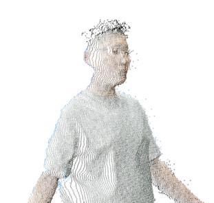
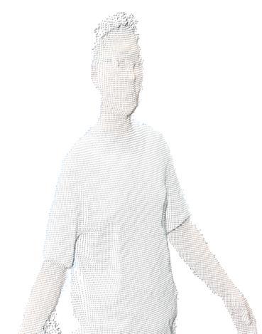
The PCA was used to filter out the outliers on two point clouds. The original point clouds are shown in Figure 3(a) and Figure 4(a), respectively.
The outliers identified by the PCA are displayed in Figure 3(b) and Figure 4(b), respectively. Figure 3(c) and Figure 4(c) are the point clouds after the outlier removal.
The basic information of the point clouds in Figure 3 and Figure 4 is listed in Table 1 below.
Table 1. Basic information of point cloud data
|
Point cloud |
Number of original data points |
Number of filtered data points |
Runtime |
|
Point cloud 1 |
26,271 |
25,510 |
2.00ms |
|
Point cloud 2 |
23,970 |
23,320 |
1.98ms |
5.2 Point cloud denoising and smoothing by bilateral filter
The point cloud denoising by the bilateral filter is the follow-up step of outlier filtering. Thus, the results of 5.1 were taken as the original data in this subsection.
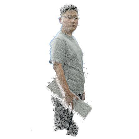
(a) Original data
(b) Noisy data
(c) Denoised data
Figure 3. Outlier correction test point cloud 1
(a) Original data
(b) Noisy data
(c) Denoised data
Figure 4. Outlier correction test point cloud 2
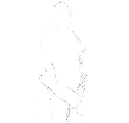
Figure 5. Filtering effect of our bilateral filter
Before using our bilateral filter, the outliers of the point clouds were removed by the PCA. The two point clouds after this denoising process are shown in Figure 5(a) and Figure 6(a), respectively. The denoised point clouds were then smoothed by our bilateral filter separately. The filtered point clouds are displayed in Figure 5(b) and Figure 6(b), respectively. Comparing the denoised images and the filtered images, it can be seen that the details of the clothes in the point clouds were obviously smoothed, especially on the sleeves; both high-frequency and low-frequency noises were removed through the combined application of the PCA and the proposed bilateral filter. The results demonstrate that our bilateral filter can retain the sharp features of point cloud data, in addition to removing the small-scale noises.
Figure 6. Filtering effect of our bilateral filter
This paper proposes a novel method to denoise the point cloud data. First, the outliers of the point cloud were removed through the PCA. Then, the denoised point cloud was smoothed by a self-designed bilateral filter, according to the vertex brightness, vertex position and normal vector. During image processing, the grayscale of the current point was replaced with the weighted mean of the grayscales of its neighborhood points. The weight function is related to the distance and grayscale difference between the current point and neighborhood points. Experimental results show that the proposed method effectively denoised and smoothed point clouds containing both high- and low-frequency noises. The results also prove that our bilateral filter can retain the sharp features of point cloud data, in addition to removing the small-scale noises. Of course, there is also some limitations with our method. The PCA assumes that all variables obey Gaussian distribution. However, some variables do not necessarily satisfy this assumption, causing scaling and rotation. This problem will be solved in future research.
This work is supported by the Youth Science Funds of National Natural Science Foundation of China (Grant No: 61702051 and 61602058); Key Science and Technology Program of Jilin Province, China (Grant No: 20180201069GX); Technology Development Plan of Jilin Province, China (Grant No: 20190103031JH and 20190201255JC). Our thanks also go to the reviewers for their comments and suggestions.
[1] Jones, T., Durand, F., Desbrun, M. (2003). Non-iterative feature-preserving mesh smoothing. ACM Transactions on Graphics, 22(3): 943-949. https://www.doi.org/10.1145/1201775.882367
[2] Cho, H., Lee, H., Kang, H., Lee, S. (2014). Bilateral texture filtering. ACM Transactions on Graphics, 33(4): 1-8. https://www.doi.org/10.1145/2601097.2601188
[3] Li, Z.L., Zhu, L.M. (2014). Envelope surface modeling and tool path optimization for five-axis flank milling considering cutter runout. Journal of Manufacturing Science and Engineering, 136(4): 041021(9pages). https://doi.org/10.1115/1.4027415
[4] Vassiliades, V., Chatzilygeroudis, K., Mouret, J.B. (2019). Using centroidal voronoi tessellations to scale up the multidimensional archive of phenotypic elites algorithm. IEEE Transactions on Image Processing, 28(8): 4177-4188. https://www.doi.org/10.1109/TIP.2019.2905991
[5] Wang, L., Yuan, B., Chen, J. (2007). Robust fuzzy c-means and bilateral point clouds denoising. International Conference on Signal Processing. IEEE. https://www.doi.org/10.1109/TEVC.2017.2735550
[6] Wu, L.S., Shi, H.L., Chen, H.W. (2016). Denoising of three-dimensional point data based on classification of feature information. Optics and Precision Engineering, 24(6): 1465-1473. https://www.doi.org/10.3788/OPE.20162406.1465
[7] Xiao, C. X., Feng, J.Q., Miao, Y.W. (2005). Geodesic path computation and region decomposition of point-based surface based on level set method. Chinese Journal of Computers, 28(2): 250-258.
[8] Collet, A., Chuang, M., Sweeney, P., Gillett, D., Sullivan, S. (2015). High-quality streamable free-viewpoint video. ACM Transactions on Graphics, 34(4): 1-13. https://www.doi.org/10.1145/2766945
[9] Yuzhen, N., Yan, Y., Wenzhong, G., Lening, L. (2018). Region-aware image denoising by exploring parameter preference. IEEE Transactions on Circuits and Systems for Video Technology, 28(9): 2433-2438. https://www.doi.org/10.1109/TCSVT.2018.2859982
[10] Dey, T.K., Goswami, S. (2004) Provable surface reconstruction from noisy samples. Computational Geometry Theory & Applications, 35(1): 124-141. https://www.doi.org/10.1016/j.comgeo.2005.10.006
[11] Annegreet, V.O., Achterberg, H.C., Vernooij, M.W., Marleen, D.B. (2018). Transfer learning for image segmentation by combining image weighting and kernel learning. IEEE Transactions on Medical Imaging, 38(1): 213-224. https://www.doi.org/10.1109/TMI.2018.2859478
[12] Digne, J., Valette, S., Chaine, R. (2017). Sparse geometric representation through local shape probing. IEEE Transactions on Visualization and Computer Graphics, 24(7): 2238-2250. https://www.doi.org/10.1109/TVCG.2017.2719024
[13] Thanou, D., Chou, P., Frossard, P. (2016). Graph-based compression of dynamic 3D point cloud sequences. IEEE Transactions on Image Processing, 25(4): 1765-1778. https://www.doi.org/10.1109/TIP.2016.2529506
[14] Anwer, A., Ali, S.S.A., Khan, A., Meriaudeau, F. (2017). Underwater 3D scene reconstruction using kinect v2 based on physical models for refraction and time of flight correction. IEEE Access, 5: 15960-15970. https://www.doi.org/10.1109/ACCESS.2017.2733003
[15] Chaudhury, A., Brophy, M., Barron, J.L. (2016). Junction-based correspondence estimation of plant point cloud data using subgraph matching. IEEE Geoscience and Remote Sensing Letters, 13(8): 1-5. https://www.doi.org/10.1109/LGRS.2016.2571121
[16] Ali, Z., Alp, O., Iwen, M.A., Selin, A. (2018). Extension of PCA to higher order data structures: An introduction to tensors, tensor decompositions, and tensor PCA. Proceedings of the IEEE, 106(8): 1341-1358. https://www.doi.org/2010.1109/JPROC.2018.2848209
[17] Namrata, V., Praneeth, N. (2018). Static and dynamic robust PCA and matrix completion: A review. Proceedings of the IEEE, 106(8): 1359-1379. https://www.doi.org/10.1109/jproc.2018.2844126
[18] Turhan, C.G., Bilge, H.S. (2017). Class-wise two-dimensional PCA method for face recognition. IET Computer Vision, 11(4): 286-300. https://doi.org/10.1049/iet-cvi.2016.0135
[19] Menon, V., Kalyani, S. (2019). Structured and unstructured outlier identification for robust PCA: A fast parameter free algorithm. IEEE Transactions on Signal Processing, 67(9): 2439-2452. https://doi.org/10.1109/TSP.2019.2905826
[20] de Oliveira Rente, P., Brites, C., Ascenso, J., Pereira, F. (2019). Graph-based static 3D point clouds geometry coding. IEEE Transactions on Multimedia, 21(2): 284-299. https://www.doi.org/10.1109/TMM.2018.2859591
[21] Vassiliades, V., Chatzilygeroudis, K., Mouret, J.B. (2017). Using centroidal voronoi tessellations to scale up the multi-dimensional archive of phenotypic elites algorithm. IEEE Transactions on Evolutionary Computation, 22(4): 623-630. https://www.doi.org/10.1109/TEVC.2017.2735550
[22] Rakhshanfar, M., Amer, M.A. (2016). Estimation of gaussian, poissonian-gaussian, and processed visual noise and its level function. IEEE Transactions on Image Processing, 25(9): 1-13. https://www.doi.org/10.1109/TIP.2016.2588320
[23] Menon, V., Kalyani, S. (2019). Structured and unstructured outlier identification for robust PCA: A fast parameter free algorithm. IEEE Transactions on Signal Processing, 67(9): 2439-2452. https://doi.org/10.1109/TSP.2019.2905826
[24] Turhan, C.G., Bilge, H.S. (2017). Class-wise two-dimensional PCA method for face recognition. IET Computer Vision, 11(4): 286-300. https://doi.org/10.1049/iet-cvi.2016.0135
[25] Tomasi, C., Manduchi, R. (1998). Bilateral filtering for gray and color images. Computer Vision, 1998. Sixth International Conference on. IEEE. https://www.doi.org/10.1109/ICCV.1998.710815
[26] De Queiroz, R., Chou, P.A. (2017). Transform coding for point clouds using a gaussian process model. IEEE Transactions on Image Processing, 26(7): 3507-3517. https://www.doi.org/10.1109//TIP.2017.2699922
[27] Morales, N., Toledo, J., Acosta, L. Javier, S. (2016). A combined voxel and particle filter-based approach for fast obstacle detection and tracking in automotive applications. IEEE Transactions on Intelligent Transportation Systems, 18(7): 1824-1834. http://www.doi.org/ 10.1109/TITS.2016.2616718
[28] Jauer, P., Kuhlemann, I., Bruder, R., Schweikard, A., Ernst, F. (2018). Efficient registration of high-resolution feature enhanced point clouds. IEEE Transactions on Pattern Analysis and Machine Intelligence, 41(5): 1102-1115. https://doi.org/10.1109/TPAMI.2018.2831670