Sandeep Kumar Singla* | Rahul Dev Garg | Om Prakash Dubey
© 2020 IIETA. This article is published by IIETA and is licensed under the CC BY 4.0 license (http://creativecommons.org/licenses/by/4.0/).
OPEN ACCESS
The purpose of this study is to investigate the computing capabilities of machine learning algorithms and remotely sensed signals to extract the agricultural information. Many techniques and models have been developed to extract information from the remotely sensed observations, but it remains an exigent problem due to the accuracy, reliability and timeliness parameters. Sugarcane yield estimation based on the temporal profile of multi-spectral Landsat-8 data has been explored in the proposed work. An initial attempt has been made in this study to select important parameters to be used as input to the machine learning method. Mean Decrease Accuracy and Mean Decrease Gini measures of random forest algorithm have been used to select the important parameters for predictive modelling. The results of the study revealed that Green Normalized Vegetation Index, Normalized Difference Vegetation Index and Land Surface Water Index performed best among other indices. Bands B2, B3, B6 and B7 of Landsat-8 recorded as top scorers. The proposed work focused on ensemble machine learning methods to optimize the correlation of historical crop yield values with spectral information. The Random Forest method exhibits a significant performance (RMSE= 1.51 t/ha and R2 = 0.94) as compared with other methods such as Classification and Regression Tree, Support Vector Regression and K-Nearest Neighbor. The proposed model based on random forest algorithm is best among all the scenarios and growth stages, whereas model based on classification and regression tree performs worst in all the cases. The proposed study indicates that the numerical value of a single spectral parameter and single-date data is not sufficient for the reliable yield estimation because it is difficult to discriminate some of the crops due to similar phenology in a particular growth period.
random forest, SVR, CART, KNN, NDVI, MDA, MDG
High-performance computing and recent development in the field of statistical analysis based on remotely sensed observations in the spatial as well as the temporal domain, leads to the optimized and effective decision making [1]. Historical and ground truth information guided by remote sensing observations has been repeatedly and effectively used to monitor the agricultural fields and other important resources [2]. Further, the extracted information and geoinformatics tools may be beneficial to automate the crop inventory process [3]. Hence, computing methods such as Digital Image Processing (DIP) and geoinformatics play an important role in the estimation of yield and crop area [4].
Predictive models based on the fusion of historical data and remote sensing observations have been successfully used since the last few decades to improve the agricultural statistics [5, 6]. Despite the developments in the technology, only a few methods exhibit a strong match between predicted yield and observed yield [7]. Basso et al. [8] presented a detailed review of crop yield estimation models and suggested using remote sensing data as an input to the forecasting model. The study also suggested the use of a simple empirical model based on the correlation between the spectral, biophysical, meteorological parameters and the crop yield. Various models have been proposed in the past to estimate the yield of different crops such as wheat, rice, maize and sugarcane. Teal et al. [9] explored that the correlation between the spectral information and corn yield was exponential. In contrast to this, Ma et al. [10] found that the power function best represented the correlation of the soybean yield and spectral data.
This work aims to develop a model based on the machine learning algorithm to predict the sugarcane yield from spectral observations. The temporal profile of spectral vegetation indices and historical crop yield records has been used as input to the underlying model to obtain a reliable estimate of the sugarcane yield. Different regression models have been developed to predict the sugarcane yield. These models have been developed on the basis of statistical analysis and extracted numerical values of vegetation indices acquired during the best predicted period.
Subsequently, the obtained information may be useful for the policy-makers and agricultural scientists to support their decisions regarding the regional agricultural risks in the near future.
Recent developments in the computing methods allowed the user to extract information with ease even from the massive amount of data. Zhu et al. [11] demonstrated deep learning model Long Short Term Memory (LSTM) for the classification of GPS data. The study also suggested the use of optimized parameters for the effective extraction of the information. The study also explored the recent methods such as Back Propagation Neural Network (BPNN), Random Forest (RF) and Convolutional Neural Networks (CNN). Relevant Component Analysis (RCA) [12] based on machine learning has been presented for the classification of remotely sensed data. The performance of RCA method was significantly better than the traditional methods. The machine learning methods may be used to extract the thematic information from the satellite data that can be employed for various domains such as Agriculture, Urban Planning, Disaster Management and Climatic studies. Various agricultural applications and operations such as yield estimation, area estimation and monitoring of the crop growth can be carried out easily under the guidance of these models and remotely sensed data [13].
Dadhwal et al. [14] discussed that the spectral data has been predominately used for the agricultural applications since the launch of the civilian remote sensing program in 1960. The paper also described Crop Identification Technology Assessment for Remote Sensing (CITARS) and Large Area Crop Inventory Experiment (LACIE) related to agricultural applications of remote sensing [15, 16]. Researchers in the past discussed recent advancements in information technology and spatial and spectral information that can assist the policy-makers in extracting the information related to the crop yields more accurately. Timely and accurate information is a prerequisite for reliable predictive modelling and efficient crop growth monitoring [17]. Nitrogen content of the plant, an indicator of the plant growth, may be estimated from Near Infrared (NIR) reflectance [18]. Spatio-temporal trend analysis of Land Surface Temperature (LST) is important to study the impact of climate change on the agricultural environment [19]. The problem of misclassification due to the spatial resolution or presence of attenuations such as clouds may affect the predictive accuracy. The problem of misclassification due to the spatial resolution or presence of attenuations such as clouds may affect the predictive accuracy. Some recent methods of bagging, boosting and stacking may significantly improve predictive accuracy [20].
Gunnula et al. [21] proved that the relationship between information and sugarcane yield is highly significant. Rahman and Robson [22] proposed a sugarcane yield prediction algorithm based on values obtained from Landsat data. The algorithm estimated the sugarcane yield with a significant correlation (R2 = 0.69).
However, sometimes the yield models based on spectral data or indices may not perform well due to the low spatial resolution or the quality of the other input data. The resolution and quality of the spectral data may be enhanced using pan sharpening algorithms, the fusion of data from multiple sources and the application of temporal profile of the available information [23].
Rao et al. [24] suggested that multi-temporal spectral data should be applied for the predictive modelling for sugarcane yield as single date imagery of Landsat data is not sufficient to participate in the model. Gers [25] developed a model based on multi-temporal Landsat data and sugarcane yield at Umfolozi in South Africa. Vo et al. [26] suggested using the temporal profile of the historical data for the predictive model based on machine learning methods K-Means Clustering and Support Vector Machine (SVM). Bégué et al. [27] presented a model based on regression with R2 value of 0.78 between the sugarcane yield and the NDVI at the ripening stage of the sugarcane. Morel et al. [28] compared various crop yield forecasting methods based on the empirical relation of NDVI values with yield records.
Researchers in the past suggested the enhancement of the model by the use of input from known crops or by the use of meteorological data and biophysical parameters. Almeida et al. [29] estimated the yield of sugarcane with an acceptable error of 1% to the actual yield. Fernandes et al. [30] proposed a model based on the decision tree with R2 value of 0.56 between sugarcane yield and multi-temporal NDVI. The model also explained the variations of NDVI values during the different development phases such as establishment, vegetative development and senescence. Rembold et al. [31] suggested the use of ground truth data with remote sensing information for the quality analysis. Marin and Jones [32] developed a process based model based on the variations in LAI of sugarcane. Mello et al. [33] proposed a technique based on spectral data from 2003 to 2012 to predict the yield with an error of 0.8%.
Ahamed et al. [34] presented a comprehensive review on the use of methods based on remotely sensed data to liberate robust, reliable, timely and accurate information. The brief review of the available literature revealed that selection and combination of appropriate spatial as well as spectral information along with suitable processing methods for the extraction of information related to sugarcane is most important, particularly for the small areas. Hence, the present work has been devoted to the use of spectral data in the temporal domain to automate the prediction of sugarcane yield. Various machine learning methods such as RF, SVR, and CART have been employed for the prediction and feature selection.
This work is focused on timely and accurate estimates about the sugarcane yield and by-products to enable the policy-makers to make decisions about the food grain production. Data and information from multiple sources are integrated to guide the analysis process further. This section is devoted to the brief details of the study area, data used and the formulae and methods used to develop the sugarcane yield model.
3.1 Datasets used for the modelling
The most important input data for models related to the yield estimation is satellite data. They become very popular in recent years because of their better spatial and spectral resolutions and their capacity to generate multi-temporal products. The data from the Landsat-8 has been used in this study. The details of the satellite images and the ancillary data used in the study have been presented in Section 4. Various vegetation indices generated from spectral bands have been investigated in the proposed work. The mathematical formulation and the brief description of each vegetation index used in the proposed model have been presented in Table 1.
Table 1. Spectral vegetation indices
|
Index |
Formula |
Ref. |
|
RVI |
$\frac{N I R_{-} r e f}{R_{-} r e f}$ |
[35] |
|
NDVI |
$\frac{\text { NIR_ref }-R_{-} r e f}{N I R_{-} r e f+R_{-} r e f}$ |
[36] |
|
SAVI |
$\frac{\left(N I R_{-} r e f-R_{-} r e f\right)(1+L)}{N I R_{-} r e f+R_{-} r e f+L}$ |
[37] |
|
GNDVI |
$\frac{N I R_{-} r e f-G_{-} r e f}{N I R_{-} r e f+G_{-} r e f}$ |
[38] |
|
OSAVI |
$\frac{\left(N I R_{-} r e f-R_{-} r e f\right)(1+L)}{N I R_{-} r e f+R_{-} r e f+0.16}$ |
[39] |
|
DVI |
$N I R_{-} r e f-R_{-} r e f$ |
[40] |
|
ARVI |
$\frac{\text { NIR_ref }-\left(\left(2 * R_{-} r e f\right)-B_{-} r e f\right)}{\text { NIR_ref }+\left(\left(2 * R_{-} r e f\right)-B_{-} r e f\right)}$ |
[41] |
|
GCI |
$\frac{N I R_{-} r e f}{G_{-} r e f}-1$ |
[42, 38] |
|
EVI |
$\frac{G\left(N I R_{-} r e f-R_{-} r e f\right)}{N I R_{-} r e f+C 1\left(R_{-} r e f\right)-C 2\left(B_{-} r e f\right)+L}$ |
[43, 44] |
|
VARI |
$\frac{G_{-} r e f-R_{-} r e f}{G_{-} r e f-R_{-} r e f-B_{-} r e f}$ |
[45] |
|
NDWI |
$\frac{G_{-} r e f-N I R_{-} r e f}{G_{-} r e f+N I R_{-} r e f}$ |
[46] |
|
NDMI |
$\frac{\text { NIR_ref }-\text { SWIR_ref }}{\text { NIR_ref }+\text { SWIR_ref }}$ |
[47] |
|
NR |
$\frac{R_{-} r e f}{\text { NIR_ref }+R_{-} \text {ref }+G_{-} \text {ref }}$ |
[48] |
|
NG |
$\frac{G_{-} r e f}{\text { NIR_ref }+R_{-} \text {ref }+G_{-} \text {ref }}$ |
[48] |
|
NN |
$\frac{\text { NIR_ref }}{\text { NIR_ref }+\text { R_ref }+G_{\text {_ref }}}$ |
[48] |
where, NIR_ref is the reflectance in the near infrared band, R_ref is the reflectance of the red band, G_ref is reflectance of the green band, B_ref is reflectance of the blue band of Landsat-8 and L is the soil and canopy adjustment constant. Normalized Difference Vegetation Index (NDVI), Green Normalized Difference Vegetation Index (GNDVI), Enhanced Vegetation Index (EVI), Soil Optimized Vegetation Index (SAVI) and its optimized version (OSAVI) are most commonly used indices for agricultural applications of remote sensing, whereas, the simplest index is Ratio Vegetation Index (RVI). These indices generally vary between -1 and +1. Atmospherically Resistant Vegetation Index (ARVI) and Visible Atmospherically Resistant Index (VARI) may be used for the correction of atmospheric scattering errors such as aerosols. Normalized Difference Moisture Index (NDMI) and Normalized Difference Water Index (NDWI) can be used for the assessment of water and moisture content in the plants and crops. NDMI is also referred as Land Surface Water Index (LSWI). These indexes are also useful to determine the Land Surface Temperature (LST) and can be employed for the irrigation management. Green Chlorophyll Index (GCI) was introduced to estimate the chlorophyll content and total pigment of a plant. Some other indices such as Normalized Green (NG), Normalized Near Infrared (NN) and Normalized Red can be used to extract the agricultural information based on the remotely sensed data. Generally, the negative values and values near to zero are specific to soil with no vegetation or sparse vegetation. In contrast the surfaces covered by dense and healthy vegetation have values 0.7 to 1.0. These vegetation indices play an important role in the extraction of thematic information from the remotely sensed data. Various crop growth, crop area estimation, crop yield estimation and crop simulation models in the recent past employed these vegetation indices as input parameters.
Sugarcane yield records and other parameters have been collected from the different agricultural fields of Khelri and Dhanauri areas in the Himalayan foothills. The area belongs to Bhadarabad region of Haridwar district in Uttarakhand State of India. The collected data has been kept for the training and testing of the underlying models in the study. Data have been collected from the State Agriculture Department, nearby sugarcane industries and by interviewing the farmers.
3.2 Feature selection
The use of remotely sensed data in the temporal domain always leads to a large number of features. The high dimensionality increases the complexity of the underlying model as well as the execution time [49]. Methods based on machine learning may be used to select and evaluate features to improve the performance of the underlying model [50]. Bocca et al. [51] discussed the importance of feature selection methods in the context of accurate and reliable sugarcane yield modelling. In addition to the reducing complexity and computational time, feature selection allows a better interpretation of the underlying model [52]. They investigated the use of Correlation-based Feature Selection (CBFS), Forward Feature Selection (FFS), Variance Inflation Factor (VIF) and Random Forest Variable Importance (RFVarImp) algorithm for the machine learning model of sugarcane yield. Their results indicate that the feature selection improves the accuracy of the model and reduces the chances of over-fitting. Hence, the minimization and optimization of the input variables are essential aspects of the development of a yield estimation model. The selection of bands and indices for the analysis based on remote sensing may be handled through the use of Principal Component Analysis (PCA) and Exploratory Factor Analysis (EFA) [53]. The proposed study applied random forest based methods for selecting important variables to generate the datasets for the model.
3.3 Regression modelling – methods and implementation
Preliminary analysis has been performed on the correlation of extracted indices from spectral data and the historical yield records from the year 2015 to 2018. The database for each crop type in the experimental area is prepared on the basis of the Pearson correlation coefficient (r). The coefficient r is the relation between the historical crop yield (y) and mean vegetation index (x) values for each crop in the temporal domain. The dates having maximum, minimum, mean and the integrated values of the corresponding index for each pixel are stored in another database. The time period associated with the maximum correlation value has been recognized as an optimal period for the prediction of crop yield.
Mathematically, the crop yield matrix for each crop ("$yield^{\text {type }}$") and the matrix containing NDVI values is given by:
$yield^{t y p e}=\left[\begin{array}{c}\text { yield }_{t_{1}} \\ \vdots \\ \text { yield }_{t_{n}}\end{array}\right]$ (1)
$x^{t y p e}=\left[\begin{array}{ccc}x_{11}^{t y p e} & \cdots & x_{1 t}^{t y p e} \\ \vdots & \ddots & \vdots \\ x_{n 1}^{t y p e} & \cdots & x_{n t}^{t y p e}\end{array}\right]$ (2)
where:
n = No. of pixels in the study area;
t = Total number of periods of the year for NDVI;
type = Crop type.
After the successful generation of the database for the regression modelling, the identification of the optimal period for the prediction of crop yield has been processed based on the random forest measures MDA and MDG. The selected periods have been used as the independent variables in the proposed regression models.
3.4 Modelling methods and implementation
Preliminary analysis has been carried out on the basis of simple models such as linear model, logarithmic model, polynomial model, exponential model and power series model. Detailed analysis based on machine learning methods SVR, CART, KNN and RF have been carried out for regression modelling. All these methods have been implemented using the open-source software “R”. The package “caret” has been used to write down the source code for the proposed regression modelling [54]. The tuning parameters for each method have been used in the proposed work to optimize the overall performance. Tuning parameter for CART is maxdepth, two parameters σ and C for SVR, one parameter k for KNN and two parameters ntree and mtry for RF.
3.5 Performance evaluation measures
Performance evaluation measures such as MAE, RMSE and R2 have been used to investigate the performance and behavior of the predictive models to estimate the sugarcane yield in the study area.
3.5.1 Root Mean Square Error (RMSE)
Statistical indicator RMSE has been used to enumerate the weighted variations between the estimated and actual yield. Mathematically, it is expressed as:
$R M S E=\sqrt{\frac{1}{n} \sum_{i=0}^{n-1}\left(p y_{i}-o y_{i}\right)^{2}}$ (3)
3.5.2 Mean Square Error (MSE)
The ground truth values and the predicted values by the underlying algorithm have been normalized in [0, 1]. The average of the square of the differences between the normalized ground truth and evaluated normalized values have been calculated using the formula:
$M S E=\frac{1}{n} \sum_{i=0}^{n-1}\left(p y_{i}-o y_{i}\right)^{2}$ (4)
3.5.3 Mean Absolute Error (MAE)
The mean of the absolute differences between the predicted and actual values has been calculated using the formula:
$M A E=\frac{1}{n} \sum_{i=0}^{n-1}\left|p y_{i}-o y_{i}\right|$ (5)
where, n is the total number of observations, py denotes estimated or predicted yield oy is the observed or actual yield. These performance evaluation metrics have been used in the different modules of the proposed model.
3.6 Algorithm for predictive model
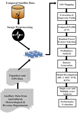
The methodology adopted to design and develop the proposed predictive model has been shown in Figure 1. The modules used in the development of the model have been represented by the following algorithm.
Algorithm 1: Proposed algorithm for Predictive Model
Module 1: Acquisition of Data:
Module 2: Pre-processing:
Module 3: Feature Selection:
Module 4: Preliminary Analysis:
Module 5: Modelling based on Machine Learning Methods:
All the modules are implemented with the help of open source software QGIS and R. The modules of the proposed algorithm have been implemented as following sub-algorithms:
Sub-Algorithm 1: Creation of LayerStack
j $\leftarrow$1
for i = 1 to n do
if image_i_meta_cloud < 20 then
Convert_DNtoRe f (Ti)
for k = 1 to 7 do
PushTi(Band_k) to LayerStack
end for
for M = 1 to 10 do
PushTi(VI_m) to LayerStack
end for
j $\leftarrow$ j + 1
end if
end for
Sub-Algorithm 2: Variable Importance
for i = 1 to j do
plotMDA(laytertack(i);)
plotMDG(laytertack(i);)
end for
optimize(ntree; mtry; oobmin)
for x = 1 to ntree do
calculateOOB(mtry; oobmin)
calculateOOB(mtry=2; oobmin)
calculateOOB(sqrt(mtry); oobmin)
end for
select ntree and corresponding mtry with minimum OOB
Sub-Algorithm 3: Yield Estimation Model
validationIndex $\leftarrow$ createDataPartition(mydata; p = 0:80)
validation $\leftarrow$ mydata[-validationIndex; ]
dataset $\leftarrow$mydata[validationIndex; ]
trnControl trainControl(method = “repeatedcv”; n = 10; rep = 3)
model.fit $\leftarrow$ train(Crop.; dataset; method=(SVR, CART,KNN, RF)
validation of model on sample data
All the modules have been implemented and the results obtained have been discussed in the next section. The performance comparison of the machine learning methods used in the proposed work has been carried out to select the best model for the prediction.
Figure 1. Flow diagram of proposed methodology
The proposed work is focused on the yield estimation of sugarcane, based on the spectral parameters and the yield records obtained during 2015, 2016, 2017, 2018 and 2019. Machine learning methods such as random forest, support vector regression, k-nearest neighbor and classification and regression tree have been tested as predictive model for the underlying work. Random forest measures MDA and MDG have been explored for the purpose of dimensionality reduction.
4.1 Extraction of spectral observations
The satellite data for the modeling activity has been obtained from the Landsat-8 and downloaded from https://earthexplorer.usgs.gov. The spectral data was obtained in the form of Digital Numbers (DN). For accurate analysis of the spectral data, the DN was converted to actual reflectance values with the help of metadata (MTL File) provided with the spectral observations. The spectral observations were received in different bands such as Blue Band, Green Band, Red Band and Near Infrared Band. After the acquisition and preprocessing of the satellite data the process for the extraction of spectral indices has been employed to extract particular and relevant information. The significance of each index has been discussed in the section 3.1. The development of the model starts with an initial phase of feature selection. Total of 40 cloud-free satellite images acquired through the entire growth seasons have been used for the analysis (Table 2). The images have been assigned the names according to the date and year of acquisition. First image acquired in 2015 has been designated as T1_1, second image as T1_2 and so on up to the image T1_6 for the last image acquired on 11th November in the year 2015. Similarly, the images for the year 2016 prefixed with T2 and the sequence number of the images (1 to 8) has been used as a suffix. The nomenclature of all the other images has been assigned in a similar manner. The spectral bands and vegetation indices extracted from these images have been provided as input to the feature selection phase.
Table 2. Landsat dataset used in the study
|
Image |
Date |
Image |
Date |
|
T1_1 |
Apr. 17, 2015 |
T3_7 |
Oct. 31, 2017 |
|
T1_2 |
May 03, 2015 |
T3_8 |
Nov. 16, 2017 |
|
T1_3 |
May 19, 2015 |
T3_9 |
Dec. 02, 2017 |
|
T1_4 |
Sep. 08, 2015 |
T4_1 |
Mar. 24, 2018 |
|
T1_5 |
Oct. 10, 2015 |
T4_2 |
Apr. 25, 2018 |
|
T1_6 |
Nov. 11, 2015 |
T4_3 |
May 11, 2018 |
|
T2_1 |
Mar. 03, 2016 |
T4_4 |
Jun. 12, 2018 |
|
T2_2 |
May 21, 2016 |
T4_5 |
Sep. 16, 2018 |
|
T2_3 |
Aug. 25, 2016 |
T4_6 |
Oct. 02, 2018 |
|
T2_4 |
Sep. 26, 2016 |
T4_7 |
Oct. 18, 2018 |
|
T2_5 |
Oct. 12, 2016 |
T4_8 |
Nov. 19, 2018 |
|
T2_6 |
Oct. 28, 2016 |
T4_9 |
Dec. 05, 2018 |
|
T2_7 |
Nov. 13, 2016 |
T5_1 |
Feb. 23, 2019 |
|
T2_8 |
Nov. 29, 2016 |
T5_2 |
Apr. 28, 2019 |
|
T3_1 |
Mar. 05, 2017 |
T5_3 |
May 30, 2019 |
|
T3_2 |
May 08, 2017 |
T5_4 |
June 15, 2019 |
|
T3_3 |
May 24, 2017 |
T5_5 |
July 01, 2019 |
|
T3_4 |
Sep. 13, 2017 |
T5_6 |
Oct. 21, 2019 |
|
T3_5 |
Sep. 29, 2017 |
T5_7 |
Nov. 06, 2019 |
|
T3_6 |
Oct. 15, 2017 |
T5_8 |
Dec. 08, 2019 |
4.2 Optimal selection of predictors
Seven spectral bands (B1 to B7) and 11 vegetation indices (DVI, GNDVI, LSWI, NDVI, NG, NN, NR, OSAVI, RVI, and SAVI) have been analyzed to select predictors. The selection process of the predictors has been performed using random forest measures MDA and MDG. The scores of both MDA and MDG have been presented in Table 3. It has been observed that both spectral bands and spectral indices have scored well during the entire growing season.
The MDA scores for the LSWI, NDVI and B4 have been on the higher side, whereas MDG scores of LSWI, B2 and B3 have been recorded at the top during the initial growing period of sugarcane (GS1). This may be due to the presence of the greenness of the ratoon plants. The vegetation indices GNDVI, LSWI, NDVI, NG and band B6 recorded higher values. On similar trends, the behavior of the different bands and indices during the growing season was distinguishable.
The overall scores of both measures have been presented in Table 3, and their comparison has been shown in Figure 2. It has been observed that performance of the band B1 remains almost at the lower level for both cases in each growing stage. This may be attributed to the fact that B1 may be effectively applicable to water related studies. Vegetation indices SAVI and OSAVI did not performed well as they are well suited for the soil related studies. The comparison of the scores revealed that GNDVI, NDVI and LSWI performed best among other indices. Bands B2, B3, B6 and B7 recorded as top scorers. Indices SAVI, OSAVI, RVI, DVI, NG, and NN as well as bands B1 and B5 have not performed well during the feature selection process. These bands and indices have been left out during the development of the yield estimation model. The top five variables from each score have been selected (represented by bold face in Table 3 under Total Score) for further analysis. Hence, the total 40 (10 variables during each growth stage) variables have been selected to participate in the model development.
Table 3. Feature selection using MDA and MDG
|
Features |
GS1 |
GS2 |
GS3 |
GS4 |
Total Score |
|||||
|
MDA |
MDG |
MDA |
MDG |
MDA |
MDG |
MDA |
MDG |
MDA |
MDG |
|
|
B1 |
0.00 |
0.33 |
0.62 |
1.69 |
1.92 |
4.95 |
0.75 |
0.65 |
3.29 |
7.61 |
|
B2 |
7.33 |
10.00 |
3.53 |
5.18 |
7.68 |
1.45 |
3.93 |
1.33 |
22.46 |
17.95 |
|
B3 |
6.48 |
9.41 |
3.96 |
4.97 |
8.15 |
1.77 |
7.19 |
0.85 |
25.78 |
17.00 |
|
B4 |
7.37 |
7.51 |
3.23 |
6.71 |
7.31 |
2.86 |
2.50 |
0.79 |
20.41 |
17.86 |
|
B5 |
5.71 |
2.45 |
5.69 |
2.95 |
3.68 |
0.00 |
6.17 |
0.82 |
21.25 |
6.22 |
|
B6 |
7.04 |
2.01 |
5.90 |
9.08 |
7.10 |
2.79 |
6.51 |
10.00 |
26.55 |
23.88 |
|
B7 |
6.65 |
2.76 |
4.34 |
4.29 |
7.59 |
1.91 |
5.94 |
7.99 |
24.52 |
16.95 |
|
DVI |
0.87 |
1.26 |
2.10 |
0.89 |
2.74 |
0.49 |
2.98 |
0.27 |
8.68 |
2.91 |
|
GNDVI |
2.49 |
1.82 |
5.96 |
8.91 |
2.17 |
4.73 |
2.34 |
2.19 |
12.96 |
17.65 |
|
LSWI |
10.00 |
9.19 |
8.54 |
7.43 |
7.53 |
2.77 |
6.69 |
2.03 |
32.75 |
21.42 |
|
NDVI |
7.79 |
2.66 |
7.40 |
3.57 |
9.07 |
3.72 |
10.00 |
1.80 |
34.26 |
11.75 |
|
NG |
2.19 |
1.73 |
9.67 |
7.34 |
2.05 |
5.97 |
3.91 |
1.45 |
17.81 |
16.49 |
|
NN |
1.41 |
0.68 |
1.19 |
0.00 |
1.79 |
5.91 |
1.45 |
0.00 |
5.84 |
6.59 |
|
NR |
1.93 |
0.60 |
4.87 |
1.72 |
1.02 |
4.91 |
3.56 |
0.63 |
11.38 |
7.86 |
|
OSAVI |
0.12 |
0.00 |
1.15 |
1.94 |
0.78 |
1.73 |
1.57 |
0.54 |
3.62 |
4.21 |
|
RVI |
0.42 |
0.78 |
0.34 |
1.42 |
2.15 |
5.30 |
0.00 |
0.57 |
2.91 |
8.07 |
|
SAVI |
1.55 |
0.40 |
0.90 |
0.34 |
1.82 |
0.82 |
1.93 |
1.14 |
6.19 |
2.70 |
Figure 2. MDA and MDG scores of feature selection
4.3 Results of preliminary analysis
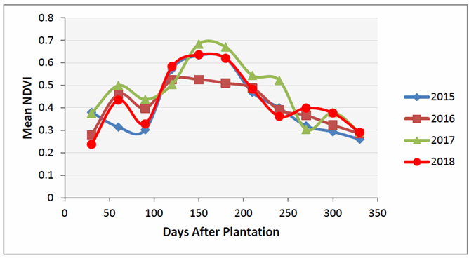
The vegetation index NDVI has been selected for the preliminary analysis for the yield estimation of sugarcane. The temporal profile of NDVI has been examined for each year of the study. The mean NDVI values from the year 2015 to 2018 for the extracted sugarcane fields in the study area have been demonstrated in Figure 3. The cavernous study of the graph revealed the increasing trend of NDVI at the initial period i.e., 50 to 55 days after the plantation (DAP). The NDVI shoots up again towards the grand growth stage and finally dips around the maturity stage.
The correlation of sugarcane yield and NDVI values has been recorded as 0.75. In contrast, the correlation of wheat and rice is below 0.6 in the area as given in Table 4. The correlation coefficient value of 0.77 has been recorded around the maturity stage of sugarcane. These observations are in agreement with the findings of Almedia et al. [29] to observe the relationship between NDVI and yield data during eight to ten months of the growing season.
Table 4. Results of correlation analysis
|
Crop Type |
Correlation Coefficient (r) |
Best Period (DAP) |
|
Sugarcane |
0.75 |
210-270 |
|
Wheat |
0.59 |
- |
|
Rice |
0.55 |
- |
Figure 3. Mean NDVI values of sugarcane fields
Regression analysis of mean NDVI (during the optimal growth period) and the historical yield records of underlying area have been presented in Table 5.
Table 5. Regression equations for the yield estimation
|
Model |
Equation |
R2 |
|
Polynomial |
$y=60.20 x^{2}-32.74 x+52.07$ |
0.555 |
|
Linear |
$y=28.19 x-36.77$ |
0.553 |
|
Exponential |
$y=38.56 e^{0.553 x}$ |
0.549 |
|
Power Series |
$y=61.71 x^{0.278}$ |
0.546 |
|
Logarithmic |
$y=14.17 \ln (x)-60.75$ |
0.550 |
Statistical analysis has been carried out to explore the significance of the results obtained from simple regression models. The most conservative multi comparison “Tukey’s Test” [55] has been implemented to carry out the analysis. The outcome of the Tukey’s test indicates that the difference between the simple regression based models was not highly significant. Hence, machine learning methods have been investigated to analyze the other indices and bands acquired during the entire growth season.
4.4 Regression modelling - machine learning methods
Preliminary analysis indicates that non-linear models may produce better results for the yield estimation. Hence, the proposed work investigated CART, KNN, RF and SVR methods of machine learning to estimate the sugarcane yield based on remotely sensed data.
The predictive models have been trained, tested and validated for the different scenarios based on the single-year and the multiple-years. Each scenario is further subdivided as per the growth stage in each year. The scenarios and their abbreviations have been given in Table 6. Machine learning modelling for the twenty-five cases (five scenarios and five stages in each scenario) has been explored in the current work. Error analysis and the relationship of predictors and yield values have been monitored for each scenario and case separately. The analysis based on different scenarios has been presented in the next section.
Table 6. Scenarios used in the modelling
|
Scenario |
Year |
Growth Stage |
|
S1 |
2015 |
Germination Stage (GS1), Tillering Stage (GS2), Grand Growth Stage (GS3), Maturity Stage (GS4), Peak of Growth (PG) |
|
S2 |
2016 |
|
|
S3 |
2017 |
|
|
S4 |
2018 |
|
|
S5 |
2015, 2016, 2017, 2018 |
4.4.1 Single-year modelling
The yield records and the spectral information acquired at each growth stage of the year 2015 have been used as inputs for the scenario S1. The outcomes of machine learning methods for scenario S1 have been presented in Table 7. It has been observed that the spectral information has been strongly correlated with yield records during the grand growth stage (GS3). Minimum values of MAE (2.20 t/ha) and RMSE (3.01 t/ha) have been recorded for the RF model. The performance of the CART model has been the lowest with a maximum value of MAE (4.65 t/ha) and RMSE (6.02 t/ha) and the lowest value of R2 (0.24). It has been ascertained from the comparative performance that the initial stages of sugarcane growing seasons are not significant for the yield estimation.
The models for the scenario S2 have been developed on the basis of data from the year 2016. The results acquired after the successful application of the model have been presented in Table 8.
Table 7. Comparative performance of scenario (S1)
|
Model |
MAE |
||||
|
GS1 |
GS2 |
GS3 |
GS4 |
PG |
|
|
SVR |
3.98 |
3.64 |
2.74 |
3.43 |
2.98 |
|
CART |
4.46 |
4.65 |
2.85 |
3.58 |
3.29 |
|
KNN |
4.19 |
3.92 |
2.67 |
3.95 |
3.06 |
|
RF |
3.46 |
3.30 |
2.20 |
3.11 |
2.57 |
|
Model |
RMSE |
||||
|
GS1 |
GS2 |
GS3 |
GS4 |
PG |
|
|
SVR |
5.39 |
5.02 |
3.73 |
4.67 |
3.90 |
|
CART |
5.75 |
6.02 |
3.70 |
4.69 |
4.30 |
|
KNN |
5.60 |
5.29 |
3.49 |
5.18 |
3.99 |
|
RF |
4.48 |
4.24 |
3.01 |
4.01 |
3.39 |
|
Model |
R2 |
||||
|
GS1 |
GS2 |
GS3 |
GS4 |
PG |
|
|
SVR |
0.21 |
0.31 |
0.63 |
0.41 |
0.59 |
|
CART |
0.19 |
0.16 |
0.61 |
0.44 |
0.48 |
|
KNN |
0.17 |
0.24 |
0.65 |
0.31 |
0.55 |
|
RF |
0.44 |
0.47 |
0.72 |
0.51 |
0.63 |
Table 8. Comparative Performance of Scenario (S2)
|
Model |
MAE |
||||
|
GS1 |
GS2 |
GS3 |
GS4 |
PG |
|
|
SVR |
3.41 |
3.33 |
2.26 |
3.41 |
2.51 |
|
CART |
3.71 |
3.86 |
2.46 |
3.58 |
2.76 |
|
KNN |
3.54 |
3.64 |
2.47 |
3.30 |
2.71 |
|
RF |
3.05 |
3.14 |
2.07 |
2.80 |
2.19 |
|
Model |
RMSE |
||||
|
GS1 |
GS2 |
GS3 |
GS4 |
PG |
|
|
SVR |
4.25 |
4.21 |
2.94 |
4.16 |
3.25 |
|
CART |
4.62 |
4.79 |
3.15 |
4.37 |
3.49 |
|
KNN |
4.36 |
4.52 |
3.04 |
4.13 |
3.44 |
|
RF |
3.84 |
4.06 |
2.66 |
3.48 |
2.87 |
|
Model |
R2 |
||||
|
GS1 |
GS2 |
GS3 |
GS4 |
PG |
|
|
SVR |
0.36 |
0.36 |
0.67 |
0.39 |
0.59 |
|
CART |
0.26 |
0.21 |
0.63 |
0.34 |
0.56 |
|
KNN |
0.32 |
0.29 |
0.65 |
0.39 |
0.57 |
|
RF |
0.46 |
0.40 |
0.73 |
0.55 |
0.68 |
The grand growth stage (GS3) is again highly correlated with the yield records of the year 2016. The best values for the performance measures are MAE (2.07 t/ha), RMSE (2.66 t/ha) and R2 (0.73), whereas the lowest performance values are MAE (3.86 t/ha), RMSE (4.79 t/ha) and R2 (0.21) respectively. The observations from the scenario S2 reveal that Grand Growth stage (GS3) and RF method is important for the yield estimation. On the other hand, the tillering stage (GS2) and CART method is the least important for the sugarcane yield estimation.
Similar results have been obtained for the year 2017 for the selection of model as well as the relationship between yield records and growth stage. However, the inferior results in terms of RMSE and MAE have been obtained. On the other hand, the R2 values have been significantly enhanced from 0.63 to 0.75, 0.61 to 0.72, 0.72 to 0.76 and 0.75 to 0.81 since year 2015. The values of the MAE, RMSE and R2 for the scenario S3 have been given in Table 9.
Table 9. Comparative performance of scenario (S3)
|
Model |
MAE |
||||
|
GS1 |
GS2 |
GS3 |
GS4 |
PG |
|
|
SVR |
3.77 |
3.77 |
2.44 |
3.65 |
2.83 |
|
CART |
4.55 |
4.56 |
2.61 |
4.28 |
3.04 |
|
KNN |
4.09 |
4.22 |
2.50 |
3.74 |
3.21 |
|
RF |
3.58 |
3.56 |
2.08 |
3.27 |
2.45 |
|
Model |
RMSE |
||||
|
GS1 |
GS2 |
GS3 |
GS4 |
PG |
|
|
SVR |
4.85 |
4.69 |
3.21 |
4.66 |
3.72 |
|
CART |
5.64 |
5.81 |
3.37 |
5.45 |
3.79 |
|
KNN |
5.22 |
5.30 |
3.17 |
4.92 |
4.14 |
|
RF |
4.69 |
4.57 |
2.73 |
4.24 |
3.19 |
|
Model |
R2 |
||||
|
GS1 |
GS2 |
GS3 |
GS4 |
PG |
|
|
SVR |
0.43 |
0.47 |
0.75 |
0.48 |
0.66 |
|
CART |
0.27 |
0.25 |
0.72 |
0.28 |
0.63 |
|
KNN |
0.35 |
0.32 |
0.76 |
0.40 |
0.57 |
|
RF |
0.47 |
0.50 |
0.81 |
0.58 |
0.74 |
Table 10. Comparative performance of scenario (S4)
|
Model |
MAE |
||||
|
GS1 |
GS2 |
GS3 |
GS4 |
PG |
|
|
SVR |
3.64 |
3.35 |
2.31 |
3.31 |
2.35 |
|
CART |
3.72 |
4.20 |
2.40 |
3.66 |
3.11 |
|
KNN |
3.83 |
3.92 |
2.49 |
3.38 |
2.79 |
|
RF |
3.06 |
3.15 |
1.97 |
2.84 |
2.25 |
|
Model |
RMSE |
||||
|
GS1 |
GS2 |
GS3 |
GS4 |
PG |
|
|
SVR |
4.87 |
4.47 |
3.24 |
4.25 |
3.32 |
|
CART |
4.88 |
5.32 |
3.23 |
4.60 |
4.34 |
|
KNN |
5.11 |
4.97 |
3.19 |
4.23 |
3.85 |
|
RF |
4.27 |
4.21 |
2.70 |
3.80 |
3.14 |
|
Model |
R2 |
||||
|
GS1 |
GS2 |
GS3 |
GS4 |
PG |
|
|
SVR |
0.31 |
0.41 |
0.70 |
0.48 |
0.69 |
|
CART |
0.36 |
0.25 |
0.70 |
0.39 |
0.50 |
|
KNN |
0.24 |
0.29 |
0.70 |
0.49 |
0.59 |
|
RF |
0.47 |
0.49 |
0.78 |
0.56 |
0.72 |
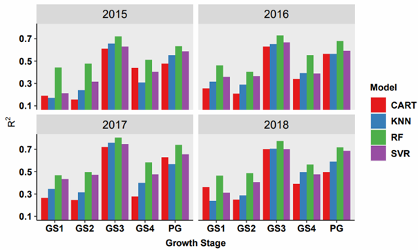
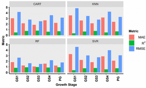
The outcomes of scenario S4 indicate that the best value of R2 (0.78) has been decreased from 0.81 obtained in the year 2017. For better analysis, these results have been validated from the validation samples. These validation samples neither belong to training samples nor to the testing. The observations of scenario S4 have been given in Table 10. The analysis based on the performance evaluation metrics (MAE, RMSE and R2) for the single-year modelling for all the scenarios have been shown in Figures 4, 5 and 6. It has been observed that the results for the years 2017 and 2018 during the grand growth stage are best, but the observations from other years are also significant. The behavior of the peak of the growth period (PG) is also significant but less than the grand growth (GS3) stage. The comparison of the methods for the modelling exhibits that the performance of the RF is best for each of the metrics. On the other hand, the performance of the CART is lowest among all the methods. The next section has been devoted to the multiple-years scenario S5.
Figure 4. MAE analysis of single-year scenarios
Figure 5. RMSE analysis of single-year scenarios
Figure 6. R2 analysis of single-year scenarios
4.4.2 Multiple-years modelling
The yield records and spectral information from the years 2015 to 2018 have been fused for multiple-year modelling. The outcomes of the model based on the scenario S5 have been given in Table 11. A comprehensive study of the outcomes indicates that the performance of the multiple-years model is significantly better than that of single-year models. The RF model is best among all the scenarios, whereas CART performs worst in all the cases, as shown in Figure 7. The MAE values have been significantly improved from the highest value of 1.97 in the year 2018 to 1.05 for multiple-years. Similarly, the RMSE values are also improved from 2.66 in the year 2016 to 1.51 and R2 values increased to 0.94 from the highest value of 0.81 in the year 2017. The RMSE and R2 values range from 1.65-3.04, 0.77-0.94 for RF models for spectral data of growth stage (GS3). Hence, the analysis based on the machine learning model reveals that the non-linear models outperformed the linear models to estimate the sugarcane yield based on the remote sensing data.
Table 11. Comparative performance of scenario (S5)
|
Model |
MAE |
||||
|
GS1 |
GS2 |
GS3 |
GS4 |
PG |
|
|
SVR |
3.26 |
2.22 |
1.84 |
2.86 |
2.11 |
|
CART |
3.02 |
2.13 |
1.85 |
2.66 |
2.22 |
|
KNN |
3.54 |
2.63 |
2.13 |
3.16 |
2.39 |
|
RF |
1.82 |
1.23 |
1.05 |
1.56 |
1.23 |
|
Model |
RMSE |
||||
|
GS1 |
GS2 |
GS3 |
GS4 |
PG |
|
|
SVR |
4.92 |
3.04 |
2.71 |
3.96 |
3.07 |
|
CART |
4.56 |
2.79 |
2.49 |
3.56 |
3.13 |
|
KNN |
5.23 |
3.43 |
2.79 |
4.21 |
3.27 |
|
RF |
2.99 |
1.65 |
1.51 |
2.18 |
1.77 |
|
Model |
R2 |
||||
|
GS1 |
GS2 |
GS3 |
GS4 |
PG |
|
|
SVR |
0.50 |
0.74 |
0.79 |
0.55 |
0.73 |
|
CART |
0.59 |
0.77 |
0.82 |
0.63 |
0.72 |
|
KNN |
0.42 |
0.66 |
0.77 |
0.49 |
0.69 |
|
RF |
0.90 |
0.93 |
0.94 |
0.88 |
0.92 |
Figure 7. Comparative analysis of multiple-year scenario
The fused data from multiple years show a significant improvement over the single-year models. The data obtained during the grand growth stages of the growing season are more important than other stages. However, the data extracted from the peak growth date, i.e., the maximum value of each spectral parameter has similar performance, but lower than that of the grand growth stage (GS3). These results may be due to the fact that yield records are highly correlated with the canopy’s vigour status. The sugarcane canopies have a stronger vigour during the grand growth stages and have a sharp increase in greenness during this period. After the grand growth period, this greenness starts converting into the sugar content and color of canopy cover changes to yellowish.
4.5 Models performance of field samples in study area
The regression models have been validated on the sample data from different fields in the study area. The sample data neither belongs to the training data nor to the testing data during the development of the model. The sample data was exploited for the analysis of differences between the predicted and the observed yield. The values obtained from the analysis of RMSE and R2 are presented through the scatter plots for different sites and different years. The scatter plots between observed and predicted sugarcane yield values for the year 2016 are shown in Figure 8. The performance of the model is low for site 2 as compared to site 1. The RMSE values for site 1 and site 2 are 1.72 (t/ha) and 2.06 (t/ha) respectively. The values for the R2 have been recorded as 0.91 and 0.85 for site 1 and site 2, respectively. The majority of the points are concentrated around the bisector line. It indicates that the model has been trained significantly for the average yield values that consistently remain between 55 to 70 in the study area.
(a) Site 1 – Dhanauri
(b) Site 2 – Khelri
Figure 8. Correlation between predicted and observed sugarcane yield for RF model on validation dataset of year 2016
A similar type of performance has been observed for the year 2017 in both the sites. RMSE values have been observed as 1.86 (t/ha) and 2.01 (t/ha) for site 1 and site 2, respectively, whereas the R2 values have been observed as 0.88 and 0.82. The obtained results for the year 2017 have been given by the Figure 9. These observations are due to the fact that there are some minor variations such as farming practice and irrigation timings. These variations in the different areas have been significantly captured by the underlying machine learning model.
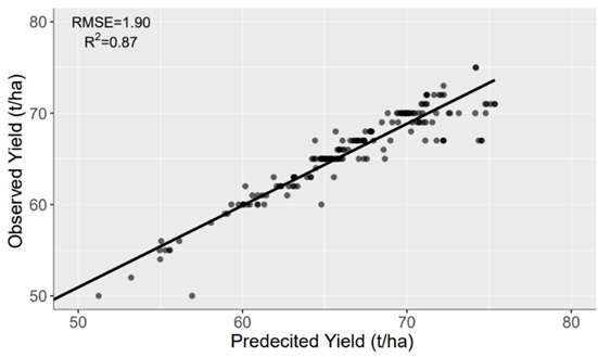
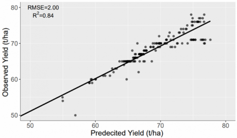
The scatter plots for the years 2018 and 2019 of both sites have been shown in Figures 10 and 11, respectively. The range of the performance indicator RMSE is between 1.72 to 1.96 (t/ha) and from 2.00 to 2.72 (t/ha) for site 1 and site 2, respectively. The range of the R2 values is between 0.87 to 0.91 for site 1 and 0.74 to 0.85 for site 2. These observations indicate that the performance of the models based on RF is quite satisfactory for both the sites.
It has been observed that the numerical value of a single spectral parameter and single-date data is not sufficient because it is difficult to discriminate some of the crops due to similar phenology in a particular growth period. Hence, in the proposed work, the single-year and multiple-years models have been developed using machine learning methods. Machine learning methods have been used to handle the variations in spectral information. These variations may be attributed to diverse agricultural practices. These include variations in soil properties, date of sowing, and variety of plants, integrated pest management, and temporal and spatial variation of crop growth. From the food management point of view, the preferable period for crop yield prediction should be as early as possible before the harvesting period. Field experimentation indicates that reliable predictions can only be made if physical phenomena of the crop growth cycle and crop yield are studied and modelled.
(a) Site 1 – Dhanauri
(b) Site 2 – Khelri
Figure 9. Correlation between predicted and observed sugarcane yield for RF model on validation dataset of year 2017
(a) Site 1 – Dhanauri
(b) Site 2 – Khelri
Figure 10. Correlation between predicted and observed sugarcane yield for RF model on validation dataset of year 2018
(a) Site 1 – Dhanauri
(b) Site 2 – Khelri
Figure 11. Correlation between predicted and observed sugarcane yield for RF model on validation dataset of year 2019
The results and their interpretations indicate that the proposed predictive model is reliable and effective for the yield estimation of sugarcane using remote sensing data. The machine learning method (Random Forest) has been found as best in comparison to other linear and non-linear models. The analysis concludes that the RF method outperforms the other methods statistically.
Sugarcane yield estimation model based on the temporal profile of spectral information of Landsat-8 has been explored in the current work. An initial attempt has been made in this study to select important parameters to be used as input to the machine learning model. Preliminary correlation and regression analysis based on NDVI values have been carried out as a pre-processing step for the final predictive model. It has been observed that non-linear models are highly significant than linear models. The optimal periods of the growing season for efficacious estimation of sugarcane yield are also identified.
Predictive models proposed in the study are focused on machine learning methods to optimize the correlation of spectral information with the available historical crop yield records. The predictive performance of the RF method is quite satisfactory for both the sites in the study area. The performance of other methods such as CART, SVM and KNN are lower as compared to the RF. Although the performance of the proposed predictive models is significant for training and testing sites, a more comprehensive estimation model may be designed by incorporating the high resolution data and more inputs from the climatic parameters.
[1] Singh, R., Semwal, D.P., Rai, A., Chhikara, R.S. (2002). Small area estimation of crop yield using remote sensing satellite data. International Journal of Remote Sensing, 23(1): 49-56. https://doi.org/10.1080/01431160010014756
[2] Vishnu Pradeep, V., Sowmya, V., Soman, K.P. (2017). Application of M-band wavelet in pansharpening. Journal of Intelligent & Fuzzy Systems, 32(4): 3151-3158. https://doi.org/10.3233/JIFS-169258
[3] Promburom, P., Jintrawet, A., Ekasingh, M. (2001). Estimating sugarcane yields with Oy-Thai interface. International Society of Sugar Cane Technologists. Proceedings of the XXIV Congress, Brisbane, Australia, Vol. 2, pp. 81-86.
[4] Panda, S.S., Ames, D.P., Panigrahi, S. (2010). Application of vegetation indices for agricultural crop yield prediction using neural network techniques. Remote Sensing, 2(3): 673-696. https://doi.org/10.3390/rs2030673
[5] Wall, L., Larocque, D., Leger, P.M. (2008). The early explanatory power of NDVI in crop yield modelling. International Journal of Remote Sensing, 29(8): 2211-2225. https://doi.org/10.1080/01431160701395252
[6] Jiang, D., Wang, N.B., Yang, X.H., Wang, J.H. (2003). Study on the interaction between NDVI profile and the growing status of crops. Chinese Geographical Science, 13(1): 62-65. https://doi.org/10.1007/s11769-003-0086-4
[7] Victoria, D.D.C., Paz, A.R.D., Coutinho, A.C., Kastens, J., Brown, J.C. (2012). Cropland area estimates using MODIS NDVI time series in the state of Mato Grosso, Brazil. Pesquisa Agropecuária Brasileira, 47(9): 1270-1278. https://doi.org/10.1590/S0100-204X2012000900012
[8] Basso, B., Cammarano, D., Carfagna, E. (2013). Review of crop yield forecasting methods and early warnings. http://www.fao.org/fileadmin/templates/ess/documents/meetings_and_workshops/GS_SAC_2013/Improving_methods_for_crops_estimates/Crop_Yield_Forecasting_Methods_and_Early_Warning_Systems_Lit_review.pdf.
[9] Teal, R.K., Tubana, B., Girma, K., Freeman, K.W., Arnall, D.B., Walsh, O., Raun, W.R. (2006). In-season prediction of corn grain yield potential using normalized difference vegetation index. Agronomy Journal, 98(6): 1488-1494. https://doi.org/10.2134/agronj2006.0103
[10] Ma, B.L., Dwyer, L.M., Costa, C., Cober, E.R., Morrison, M.J. (2001). Early prediction of soybean yield from canopy reflectance measurements. Agronomy Journal, 93(6): 1227-1234. https://doi.org/10.2134/agronj2001.1227
[11] Zhu, S., Sun, H., Duan, Y., Dai, X., Saha, S. (2020). Travel mode recognition from GPS data based on LSTM. Computing and Informatics, 39(1-2): 298-317. https://doi.org/10.31577/cai_2020_1-2_298
[12] Zhao, H., Lu, L., Yang, C., Guan, R. (2017). Kernel feature extraction for hyperspectral image classification using Chunklet constraints. Computing and Informatics, 36(1): 205-222.
[13] Prasad, A.K., Chai, L., Singh, R.P., Kafatos, M. (2006). Crop yield estimation model for Iowa using remote sensing and surface parameters. International Journal of Applied Earth Observation and Geoinformation, 8(1): 26-33. https://doi.org/10.1016/j.jag.2005.06.002
[14] Dadhwal, V.K., Singh, R., Dutta, S., Parihar, J.S. (2002). Remote sensing based crop inventory: A review of Indian experience. Tropical Ecology, 43(1): 107-122.
[15] Bauer, M.E., Cary, T.K., Davis, B.J., Swain, P.H. (1975). Crop Identification Technology Assessment for Remote Sensing (CITARS). NASA-CR-147389, LARS-INFORM-NOTE-072175, pp. 1-59.
[16] Bauer, M.E., McEwen, M.C., Malila, W.A., Harlan, J.C. (1979). Design, implementation and results of LACIE field research. Purdue University, LARS Technical Report, 102579.
[17] Waldner, F., Canto, G.S., Defourny, P. (2015). Automated annual cropland mapping using knowledge-based temporal features. ISPRS Journal of Photogrammetry and Remote Sensing, 110: 1-13. https://doi.org/10.1016/j.isprsjprs.2015.09.013
[18] Afandi, S.D., Herdiyeni, Y., Prasetyo, L.B., Hasbi, W., Arai, K., Okumura, H. (2016). Nitrogen content estimation of rice crop based on Near Infrared (NIR) reflectance using Artificial Neural Network (ANN). Procedia Environmental Sciences, 33: 63-69. https://doi.org/10.1016/j.proenv.2016.03.057
[19] Wang, N., Xia, J., Yin, J., Liu, X. (2016). Trend analysis of land surface temperatures using time series segmentation algorithm. Journal of Intelligent & Fuzzy Systems, 31(2): 1121-1131. https://doi.org/10.3233/JIFS-169041
[20] Li, D.W., Yang, F.B., Wang, X.X. (2015). Crop region extraction of remote sensing images based on fuzzy ARTMAP and adaptive boost. Journal of Intelligent & Fuzzy Systems, 29(6): 2787-2794. https://doi.org/10.3233/IFS-151983
[21] Gunnula, W., Kosittrakun, M., Righetti, T.L., Weerathaworn, P., Prabpan, M. (2011). Normalized difference vegetation index relationships with rainfall patterns and yield in small plantings of rain-fed sugarcane. Australian Journal of Crop Science, 5(13): 1845-1851.
[22] Rahman, M.M., Robson, A.J. (2016). A novel approach for sugarcane yield prediction using Landsat time series imagery: A case study on Bundaberg region. Advances in Remote Sensing, 5(2): 93-102. https://doi.org/10.4236/ars.2016.52008
[23] Luo, X., Wu, X., Zhang, Z. (2014). Regional and entropy component analysis based remote sensing images fusion. Journal of Intelligent & Fuzzy Systems, 26(3): 1279-1287.
[24] Rao, P., Rao, V., Venkataratnam, L. (2002). Remote sensing: A technology for assessment of sugarcane crop acreage and yield. Sugar Tech, 4(3-4): 97-101. https://doi.org/10.1007/BF02942689
[25] Gers, C.J. (2003). Relating remotely sensed multi-temporal Landsat 7 ETM+ imagery to sugarcane characteristics. In: Proc S Afr Sug Technol Ass, pp. 313-321.
[26] Vo, V., Luo, J., Vo, B. (2016). Time series trend analysis based on K-means and support vector machine. Computing and Informatics, 35: 111-127.
[27] Bégué, A., Lebourgeois, V., Bappel, E., Todoroff, P., Pellegrino, A., Baillarin, F., Siegmund, B. (2010). Spatio-temporal variability of sugarcane fields and recommendations for yield forecast using NDVI. International Journal of Remote Sensing, 31(20): 5391-5407. https://doi.org/10.1080/01431160903349057
[28] Morel, J., Todoroff, P., Bégué, A., Bury, A., Martiné, J.F., Petit, M. (2014). Toward a satellite-based system of sugarcane yield estimation and forecasting in smallholder farming conditions: A case study on Reunion Island. Remote Sensing, 6(7): 6620-6635. https://doi.org/10.3390/rs6076620
[29] Almeida, T.I.R., Filho, C.R.D.S., Rossetto, R. (2006). ASTER and Landsat ETM+ images applied to sugarcane yield forecast. International Journal of Remote Sensing, 27(19): 4057-4069. https://doi.org/10.1080/01431160600857451
[30] Fernandes, L.J., Rocha, J.V., Lamparelli, R.A.C. (2011). Sugarcane yield estimates using time series analysis of spot vegetation images. Scientia Agricola, 68: 139-146.
[31] Rembold, F., Atzberger, C., Savin, I., Rojas, O. (2013). Using low resolution satellite imagery for yield prediction and yield anomaly detection. Remote Sensing, 5(4): 1704-1733. https://doi.org/10.3390/rs5041704
[32] Marin, F.R. Jones, J.W. (2014). Process-based simple model for simulating sugarcane growth and production. Scientia Agricola, 71(1): 1-16. https://doi.org/10.1590/S0103-90162014000100001
[33] Mello, M.P., Atzberger, C., Formaggio, A.R. (2014). Near real time yield estimation for sugarcane in Brazil combining remote sensing and official statistical data. 2014 IEEE Geoscience and Remote Sensing Symposium, Quebec City, QC, pp. 5064-5067. https://doi.org/10.1109/IGARSS.2014.6947635
[34] Ahamed, T., Tian, L., Zhang, Y., Ting, K. (2011). A review of remote sensing methods for biomass feedstock production. Biomass and Bioenergy, 35(7): 2455-2469. https://doi.org/10.1016/j.biombioe.2011.02.028
[35] Jordan, C.F. (1969). Derivation of leaf-area index from quality of light on the forest floor. Ecology, 50(4): 663-666. https://doi.org/10.2307/1936256
[36] Rouse, J.W., Haas, H., R., Schell, A., J., Deering, D. W. (1974). Monitoring vegetation systems in the great plains with ERTS. NASA Special Publication, 351: 309.
[37] Huete, A.R. (1988). A soil-adjusted vegetation index (SAVI). Remote Sensing of Environment, 25(3): 295-309. https://doi.org/10.1016/0034-4257(88)90106-X
[38] Gitelson, A.A., Kaufman, Y.J., Merzlyak, M.N. (1996). Use of a green channel in remote sensing of global vegetation from EOS-MODIS. Remote Sensing of Environment, 58(3): 289-298. https://doi.org/10.1016/S0034-4257(96)00072-7
[39] Rondeaux, G.R., Steven, M., Baret, F. (1996). Optimization of soil-adjusted vegetation indices. Remote Sensing of Environment, 55(2): 95-107.
[40] Tucker, C.J. (1979). Red and photographic infrared linear combinations for monitoring vegetation. Remote Sensing of Environment, 8(2): 127-150. https://doi.org/10.1016/0034-4257(79)90013-0
[41] Kaufman, Y.J., Tanre, D. (1992). Atmospherically resistant vegetation index (ARVI) for EOS-MODIS. IEEE Transactions on Geoscience and Remote Sensing, 30(2): 261-270. https://doi.org/10.1109/36.134076
[42] Gitelson, A.A., Grits, Y., Merzlyak, M.N. (2003). Relationships between leaf chlorophyll content and spectral reflectance and algorithms for non-destructive chlorophyll assessment in higher plant leaves. Journal of Plant Physiology, 160(3): 271-282. https://doi.org/10.1078/0176-1617-00887
[43] Huete, A., Justice, C., Liu, H. (1994). Development of vegetation and soil indices for MODIS-EOS. Remote Sensing of Environment, 49(3): 224-234. https://doi.org/10.1016/0034-4257(94)90018-3
[44] Huete, A., Didan, K., Miura, T., Rodriguez, E., Gao, X., Ferreira, L.G. (2002). Overview of the radiometric and biophysical performance of the MODIS vegetation indices. Remote Sensing of Environment, 83(1-2): 195-213. https://doi.org/10.1016/S0034-4257(02)00096-2
[45] Gitelson, A.A., Stark, R., Grits, U., Rundquist, D., Kaufman, Y., Derry, D. (2002). Vegetation and soil lines in visible spectral space: A concept and technique for remote estimation of vegetation fraction. International Journal of Remote Sensing, 23(13): 2537-2562. https://doi.org/10.1080/01431160110107806
[46] McFeeters, S.K. (1996). The use of the Normalized Difference Water Index (NDWI) in the delineation of open water features. International Journal of Remote Sensing, 17(7): 1425-1432. https://doi.org/10.1080/01431169608948714
[47] Wilson, E.H. Sader, S.A. (2002). Detection of forest harvest type using multiple dates of Landsat TM imagery. Remote Sensing of Environment, 80(3): 385-396. https://doi.org/10.1016/S0034-4257(01)00318-2
[48] Sripada, R., Heiniger, R., White, J., Meijer, A. (2006). Aerial color infrared photography for determining early in-season nitrogen requirements in corn. Agronomy Journal, 98(4): 968-977. https://doi.org/10.2134/agronj2005.0200
[49] Gonzalez-Sanchez, A., Frausto-Solis, J., Ojeda-Bustamant, W. (2014). Attribute selection impact on linear and nonlinear regression models for crop yield prediction. The Scientific World Journal, 2014: 1-10. https://doi.org/10.1155/2014/509429
[50] Darena, F., Zizka, J. (2013). Approaches to samples selection for machine learning based classification of textual data. Computing and Informatics, 32: 949-967.
[51] Bocca, F.F., Henrique, L., Rodrigues, A. (2016). The effect of tuning, feature engineering, and feature selection in data mining applied to rainfed sugarcane yield modelling. Computers and Electronics in Agriculture, 128: 67-76. https://doi.org/10.1016/j.compag.2016.08.015
[52] Gopal, P.S.M., Bhargavi, R. (2019). Performance evaluation of best feature subsets for crop yield prediction using machine learning algorithms. Applied Artificial Intelligence, 33(7): 621-642. https://doi.org/10.1080/08839514.2019.1592343
[53] Lavanya, A., Sanjeevi, S. (2013). An improved band selection technique for hyperspectral data using factor analysis. Journal of Indian Society of Remote Sensing, 41: 199-211. https://doi.org/10.1007/s12524-012-0214-7
[54] Kuhn, M. (2008). Building predictive models in R using the caret package. Journal of Statistical Software, 28(5): 1-26.
[55] Tukey, J.W. (1997). Exploratory Data Analysis. Addison-Wesley.